Introduction
A spectral gap is one of the principal analytic inputs in the mathematical definition of a zero-temperature quantum phase. It controls adiabatic transport, protects low-energy information, supports clustering statements, and allows topological invariants to remain locally constant along a family. It is also a frequent source of hidden assumptions. A finite matrix has a positive difference between distinct eigenvalues, but that observation says nothing about a lower bound uniform in system size. A family can have a positive gap at every parameter while its infimum is zero. A bulk GNS Hamiltonian can be gapped while open boundaries carry gapless modes.
These distinctions become unavoidable in a condensed-mathematics formulation of phases. A condensed or profinite test object can encode a family of interactions. Sheaf descent can glue compatible local descriptions. Neither operation proves that the thermodynamic generator has an isolated ground sector. The gap must remain a witnessed analytic property.
This paper addresses the third analytic problem in a five-paper program:
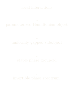
The paper does not construct the final spectrum. It supplies a defensible meaning for the third line and explains which established stability results can be imported.
Contributions
Our contributions are the following.
We give separate definitions for literal finite-volume gaps, ground-band gaps, uniform finite-volume gaps, GNS bulk gaps, and uniform parameterized GNS gaps.
We prove an elementary compactness theorem for a constant-rank isolated spectral cluster and show why rank change invalidates the common compactness shortcut.
We give three explicit counterexamples: a norm-continuous compact matrix family with pointwise but nonuniform literal gaps, a locally continuous profinite spin family with uniform locality but collapsing GNS gaps, and a sequence of finite ferromagnetic chains whose gaps close in the thermodynamic limit.
We formulate a fibration of quantitative gap witnesses and its propositional image inside the Hamiltonian functor. The witness records enough data to make the predicate meaningful and stable under restriction of the parameter object.
We separate two established analytic mechanisms. Spectral flow transports a low-energy sector along a path already known to have a uniform isolated band. Perturbative gap stability preserves a pre-existing gap only under substantive structural hypotheses such as frustration freeness, quantitative local gaps, and LTQO.
We state formalization contracts for Lean and executable finite-model checks for Haskell. These artifacts represent hypotheses and finite calculations. They do not claim proofs of infinite-volume theorems.
Status vocabulary
We use five labels throughout:
| Label | Meaning |
|---|---|
| established | A cited theorem or standard construction under stated assumptions. |
| proposed | A definition or moduli construction introduced here. |
| conjectural | A precise assertion not proved here. |
| open | No proof or counterexample is known in the stated scope. |
| obstructed | A theorem or explicit counterexample rules out the claim. |
The distinction is important. Formal vocabulary should expose uncertainty, not conceal it.
Quantum lattice framework
Local and quasi-local observables
Let be a countable metric space. We assume uniform local finiteness when a volume-growth estimate is required. Each site carries a finite-dimensional Hilbert space . For a finite set , define
If , the canonical inclusion is
These maps are unital and isometric. The local algebra and its C*-completion are
Definition 1 (Interaction). An interaction is a map such that . Its finite-volume Hamiltonian on is
The formal infinite sum of all interaction terms is generally not an element of . Under decay hypotheses, the thermodynamic object is instead a strongly continuous automorphism group, often defined first on local observables and then extended.
F-functions and uniform locality
Definition 2 (F-function). A nonincreasing function is an F-function on if and For thermodynamic limits on a general countable metric space, we also require the uniform tail condition This condition is automatic for the standard translation-invariant lattice examples used below. On , translation invariance makes the sum independent of the base point , so it is the ordinary tail of a convergent series. We state the condition separately because pointwise summability is not a substitute for a family-uniform tail on arbitrary geometry.
For an interaction , set
Standard choices on are a sufficiently fast polynomial tail and its exponentially weighted version,
Definition 3 (Uniformly local parameter family). Let be a topological parameter space. A family is uniformly F-local if It is locally F-continuous if its restrictions to every fixed finite region vary continuously in the corresponding restricted interaction norm.
Local F-continuity is a finite-region condition. It does not include the separate geometric hypothesis , which will be stated whenever a family-uniform thermodynamic limit is used.
Uniform locality and parameter continuity are distinct. Global norm continuity on compact implies uniform boundedness. It is often too strong for product-topology disorder because a change far from a fixed observation region can remain large in a supremum over all sites.
Uniform Lieb-Robinson control
The standard Lieb-Robinson argument yields a bound whose constants depend on the F-function, the geometry, and . A uniform family bound therefore gives constants independent of .
Theorem 4 (Uniform family Lieb-Robinson estimate). Assume . Let and have finite disjoint supports. For finite , The same right side works for every .
Proof status. This is an established uniform-family corollary of the usual interaction-norm Lieb-Robinson theorem. The proof is the standard iterated commutator estimate. Every occurrence of the interaction norm is bounded by the common constant . We do not claim a new proof of the sharp boundary form of the estimate. ◻
Corollary 5 (Uniform thermodynamic dynamics). Under the assumptions of theorem 2.4, and with the additional uniform-tail hypothesis , finite-volume dynamics converge on local observables along any regular exhaustion. The convergence is uniform in and on compact time intervals. If the family is also locally F-continuous, the map is norm-continuous for every local .
Proof sketch. Compare dynamics in two nested volumes by a Duhamel expansion. The difference is bounded by a common F-tail outside the smaller region, multiplied by the uniform exponential factor from theorem 2.4. Summability of and the separately assumed limit make this tail vanish uniformly in the base point. The same estimate separates a parameter variation inside a large finite region from the common tail outside it. ◻
Warning 6. Neither theorem 2.4 nor theorem 2.5 contains a gap hypothesis or a gap conclusion. Uniform causal control and a uniform spectral gap are logically separate properties.
Five gap predicates
Literal finite-volume ground-state gap
Let be self-adjoint on the finite-dimensional Hilbert space for . Write
Definition 7 (Literal ground-state gap). The literal finite-volume ground-state gap is with the convention that every eigenvector at exactly belongs to the ground space.
This definition is sensitive to a low-energy level that approaches the ground energy and becomes exactly degenerate in a limit.
Finite-volume ground-band gap
Definition 8 (Selected ground-band gap). Choose a compact interval whose intersection with the spectrum is the selected low-energy cluster, and assume that the complementary spectral set is nonempty. Define The rank of the selected spectral projection is part of the convention.
This is the natural finite-volume predicate for spectral flow. An isolated low-energy band can survive small internal splittings even when the literal ground-state gap becomes small.
Uniform finite-volume gap
Definition 9 (Uniform finite-volume band gap). Fix an exhaustion , a boundary convention, and selected bands . A family has uniform finite-volume gap if
The exhaustion and boundary convention cannot be suppressed. Open and periodic volumes can display different low-energy behavior.
GNS bulk gap
Let be an infinite-volume ground state for the dynamics . Let be its GNS triple. The dynamics is implemented by a positive generator with [BratteliRobinson2].
Definition 10 (GNS bulk gap). The GNS gap of the selected ground state is
If the GNS ground vector is unique, the positive gap can be expressed through a Poincare-type estimate on the domain of the generator. The representation and state remain essential data.
Uniform parameterized GNS gap
Definition 11 (Uniform bulk-gapped family). A family of interactions with selected ground states is uniformly bulk-gapped if there is such that
Pointwise positivity of is not enough. Uniformity is a separate quantifier and is the physically relevant one for a single parameterized phase object.
Compactness: valid theorem and invalid shortcut
Compactness does produce a common separation for a finite-dimensional spectral cluster when its rank is fixed. The rank condition is the missing hypothesis in a common but invalid argument.
Proposition 12 (Compact constant-rank spectral separation). Let be compact and let be norm-continuous. Suppose there is a continuous family of rank- spectral projections and that for every . Then the distance between the two spectral clusters has a positive minimum on .
Proof. The ordered eigenvalues of a self-adjoint matrix are Lipschitz continuous in the operator norm. After choosing which eigenvalues form the cluster, the distance between the two finite sets of continuous eigenvalue functions is a continuous positive function on . A positive continuous function on a compact space has a positive minimum. ◻
Example 13 (Rank change destroys the conclusion). Let and This is a norm-continuous family. At , the literal ground-state gap is . At , the ground space has rank two and the literal gap is . Every fiber is literally gapped, but If the two lowest levels are selected as one band, the band gap is uniformly positive. The disagreement is not a paradox. The two predicates encode different low-energy sectors.
Corollary 14. Compactness plus pointwise literal gappedness does not imply a uniform literal gap when the ground-state rank changes.
Thermodynamic counterexamples
A moving weak defect
Let with one qubit at each site. Let . Consider the product interactions whose formal Hamiltonians are
The parameter space is profinite. On every fixed finite region, agrees with for all sufficiently large . The family is locally continuous and uniformly finite range. Its Lieb-Robinson constants can therefore be chosen uniformly.
Proposition 15 (Uniform locality without a uniform gap). Each system above has the same unique product ground state. Its GNS excitation gap is Hence
Proof. A single spin flip at site has energy for , and every nonzero excitation has energy at least . For , a single spin flip has energy and all other excitations have integer energy at least . ◻
The family is not continuous in the global interaction norm that takes a supremum over all sites. This example explains why local parameter continuity and uniform locality should be stated separately.
Finite chains with a closing gap
For a length- open spin- ferromagnetic chain, let
where swaps neighboring spins. Each summand is positive and the model is frustration free.
Proposition 16 (Finite positivity does not imply a thermodynamic gap). Every finite has a positive gap above its symmetric ground space, but
Proof sketch. Restrict to the one-magnon sector. There the Hamiltonian is proportional to the graph Laplacian of the length- path. Its first nonzero eigenvalue is in the stated normalization. The variational principle gives the upper bound on the full many-body gap. ◻
The infinite isotropic ferromagnetic chain is gapless. A theorem about all finite volumes must contain a lower bound independent of if it is to imply a thermodynamic gap.
Spectral flow transports an assumed gap
Quasi-adiabatic continuation relates uniformly gapped paths to quasi-local automorphisms. It is a transport theorem, not a gap-existence theorem.
Hypotheses
Let be differentiable for . The standard finite-volume-to-thermodynamic spectral-flow theorem assumes, in a typical form:
finite-dimensional local spin spaces;
a regular exhaustion with controlled geometry;
a decay norm for and bounded uniformly in ;
a selected finite-volume spectral interval ;
a separation between that interval and the rest of the spectrum, uniform in and .
Choose a filter adapted to the gap. The finite-volume generator is
The decay of the filter and the Lieb-Robinson estimate make this generator quasi-local.
Theorem 17 (Thermodynamic spectral flow). Under the stated locality, differentiability, geometry, and uniform ground-band gap assumptions, the finite-volume flows converge to a strongly continuous cocycle of quasi-local automorphisms of . The thermodynamic ground-state sets satisfy
Proof status. This is the established automorphic-equivalence theorem of Bachmann, Michalakis, Nachtergaele, and Sims, stated here in the notation of this paper. The proof combines a filtered quasi-adiabatic generator, quasi-locality bounds, uniform convergence, and transport of the isolated spectral projection. ◻
Warning 18 (No circular use). The uniform gap is an input to the filter and to the spectral projection transport. Theorem 6.1 cannot be cited to prove that the same path has a gap.
Bulk spectral-flow variants
There are bulk formulations based on a unique selected ground state with a uniform GNS gap and suitable differentiability estimates. These avoid treating open-boundary low-energy modes as bulk gap closure. They still assume the bulk gap. They do not establish general perturbative stability.
Controlled perturbative gap stability
General stability of the spectral gap for arbitrary interacting Hamiltonians is not available. Strong theorems exist for structured classes. We describe a representative frustration-free lane.
Frustration-free reference system
Assume an interaction indexed by sites,
where is supported in a ball of common finite radius, , and the selected infinite-volume state has zero energy on every local term.
Let be the positive GNS generator. A stability theorem starts with
This is a pre-existing bulk gap, not a consequence of frustration freeness.
Local gap control
For controlled local regions , assume a polynomial lower bound on the local gap,
for constants and . The local gap may decay, but its decay is quantified.
Local Topological Quantum Order
Let project onto the local ground space in a ball of radius . A representative LTQO estimate is
for supported in and . The decay function must have enough finite moments relative to the spatial growth, partition growth, and local-gap exponent.
This estimate says that local ground states become indistinguishable by an observable sufficiently far from the boundary. Its quantitative form is essential to the perturbative argument.
Anchored perturbations
Write the perturbation as an anchored interaction
with stretched-exponential decay
Theorem 19 (Controlled bulk gap stability). Assume regular polynomial geometry, a finite-range positive frustration-free reference interaction, a selected GNS sector whose vacuum vector is nondegenerate for the implementing bulk generator, a positive bulk GNS gap , quantitative local gap control, LTQO with the required decay moments, and a stretched-exponentially decaying anchored perturbation. For every , there is a perturbation threshold such that preserves a unique transported ground state and a GNS gap at least .
Proof status. This is an established theorem in the Nachtergaele-Sims-Young stability framework. The proof uses spectral flow to conjugate the perturbed Hamiltonian into a form whose ground-state contribution is controlled by LTQO, while the local gap bounds dominate the remaining relatively bounded terms. We state the hypothesis package because omitting any part would suggest a false theorem for arbitrary gapped systems. ◻
Remark 20 (Finite-volume topological degeneracy). Nondegeneracy in theorem 7.1 refers to the vacuum vector in the selected infinite-volume GNS sector. It does not assert that the local ground projections have rank one. LTQO is designed to control locally indistinguishable finite-volume ground spaces, including topologically degenerate ones.
Remark 21. Earlier finite-volume stability results of Michalakis and collaborators provide a closely related LTQO lane. Precise assumptions differ between formulations. A paper must cite the version it actually uses.
What the theorem does not prove
Theorem 7.1 does not apply automatically to:
arbitrary frustrated Hamiltonians;
power-law interactions outside the allowed decay class;
reference systems without a known bulk gap;
models lacking local gap control or LTQO;
families in which the symmetry or ground-state convention changes;
claims about all open-boundary spectra.
Witness fibration and qualitative gapped subfunctor
We now state the moduli proposal. It is designed so that gap data cannot be lost by notation.
Hamiltonian family object
Let be a compact Hausdorff or profinite test object. Define schematically
Additional data records symmetry, on-site Hilbert spaces, and the allowed coarse geometry. The assignment should be treated as a groupoid or higher stack once unitary equivalences and automorphisms are included.
Gap witness
Definition 22 (Gap witness). A gap witness for consists of:
a declared gap predicate, either finite-volume band or GNS bulk;
an exhaustion and boundary convention in the finite-volume case;
a selected spectral band of locally constant rank, or selected ground states in the GNS case;
a common number ;
verification that the selected predicate is at least for all and all required volumes;
continuity data for the selected projections or states sufficient for the later phase equivalence.
Define the quantitative witness object
The projection forgets the witness. It is not generally injective because one family can have many lower bounds, states, exhaustions, or theorem providers. Thus the witnessed object is a fibration of data over the Hamiltonian functor, not a subfunctor in the monomorphism sense.
Define the qualitative gapped image by propositional existence: Here means that only existence is retained. Equivalently, take the image of . The qualitative object is a subfunctor of when image formation and pullback are implemented in the chosen sheaf or stack category. Both constructions are proposed.
Proposition 23 (Restriction stability). Let be continuous. Pullback of a witnessed family along preserves the common lower bound and defines a witnessed family over .
Proof. The pulled-back family is indexed by . The uniform locality bound over is no larger than the bound over . Every selected gap is one of the gaps already bounded below on , so the same works. Pull back the state, band, and continuity data componentwise. ◻
Descent is not gap creation
Suppose a finite jointly surjective family covers the parameter object. Compatible interaction families can descend. If every local witness comes with the same explicit lower bound and compatible state or band data, the witness can also descend in a controlled formulation.
It is invalid to assume only that every restriction has some unspecified positive lower bound. The minimum is available for a finite cover, but the selected bands and states must agree on overlaps. For varying or infinite covers, further uniformity is required. Sheaf descent organizes compatible evidence. It does not produce evidence that was not supplied.
If gapped neighborhoods form an open cover of a compact parameter space, then compactness provides a finite subcover. Compatible quantitative witnesses on that finite subcover yield a common positive minimum. This argument still requires one fixed predicate and compatible state or band conventions. A bare pointwise statement need not provide such neighborhoods or compatibility.
Openness and discriminant locus
For a norm-continuous finite matrix family with a fixed-rank isolated cluster, gappedness is open. For interacting thermodynamic families, openness follows only inside a class covered by a stability theorem.
Given a parameter map , define the witnessed gapped locus
and the gapless discriminant
On underlying parameter sets or spaces, this pullback is a genuine subobject, so its complement is meaningful. The larger pullback with is instead a bundle of witnesses over and must not be subtracted from . The notation is meaningful only after the gap predicate, image construction, and witness category are fixed. A topological phase label is expected to be locally constant on after quotienting by the chosen stable gapped equivalences.
Relations among the predicates
The following table summarizes safe implications.
| Statement | Status and qualification |
|---|---|
| Uniform finite-volume gap implies a bulk GNS gap | established in controlled limits with stated uniqueness, regularity, and boundary assumptions. Not a definition-level implication. |
| Bulk GNS gap implies open-boundary finite-volume gap | obstructed in general by topological boundary modes. |
| Every finite volume is gapped implies a thermodynamic gap | obstructed by the ferromagnetic-chain example. |
| Pointwise parameter gaps imply a common gap | obstructed without constant-rank or stability hypotheses. |
| Uniform locality implies a uniform gap | obstructed by the moving weak-defect example. |
| Uniform gapped path implies quasi-local automorphic transport | established under spectral-flow locality and regularity assumptions. |
| Small perturbations preserve an arbitrary interacting gap | open as a universal theorem; established only for controlled structural classes. |
Worked finite examples
Two-level constant-rank family
Let
The eigenvalues are , so the separation is . The negative spectral projection has constant rank one. This is the elementary setting where compactness and continuity correctly produce a common gap.
A stable product-spin perturbation
For qubits, consider
with and commuting diagonal . If every excited on-site level remains at least above the local ground level, then the many-body product gap is at least , independent of . This direct estimate uses the product and commuting structure. It is not a general theorem for noncommuting perturbations.
Bulk and boundary conventions
An open topological chain can have boundary modes with a splitting that vanishes exponentially in length, while the periodic bulk has a stable gap. The literal open-chain ground-state gap, the open-chain ground-band gap, and the bulk GNS gap answer different questions. A phase definition intended to ignore protected edge degeneracy should use a band or bulk predicate and say so explicitly.
Formal and executable representations
Lean theorem interfaces
A Lean library can honestly represent the logical dependency graph without formalizing the full analytic proofs. It should contain:
finite sites, finite supports, and finite-volume Hamiltonian data;
a parameter family and a predicate expressing a common norm bound;
literal finite-spectrum gaps and selected-band gaps;
a structure containing a positive common gap witness;
an abstract GNS-gap predicate whose provider is an explicit interface;
an abstract spectral-flow provider that requires a uniform gap witness;
an abstract stability provider that lists LTQO and local-gap inputs;
status and provenance fields for each imported analytic result.
The preferred design uses structures and theorem-provider typeclasses rather than global axioms. A concrete development can instantiate the interface when the relevant theorem has been formalized. No declaration should suggest that Lean proved an infinite-volume spectral gap merely because a finite list of eigenvalues was checked.
Haskell demonstrations
Executable code accompanying this paper checks finite calculations:
ordered-spectrum gap extraction;
selected-band separation;
the matrix family in theorem 4.2;
the closing upper bound for the ferromagnetic chain;
finite prefixes of the moving weak-defect gap sequence;
predicates distinguishing pointwise positivity from a declared common lower bound.
These checks are computational. They catch convention and implementation errors. They are not thermodynamic proofs.
Main results in concise form
We collect the paper’s conclusions.
Theorem 24 (Separation theorem). Uniform F-locality, local parameter continuity, and pointwise positive GNS gaps do not imply a parameter-uniform GNS gap, even for a profinite family of finite-range commuting product interactions with a common unique ground state.
Proof. The moving weak-defect family supplies all stated properties and has gaps along a sequence converging to the parameter . ◻
Theorem 25 (Witness necessity). Any moduli assignment that records only an interaction family and the statement that each fiber is gapped cannot distinguish the moving weak-defect family from a uniformly gapped family. A uniform phase subobject must therefore record or require a common quantitative lower bound, together with the gap convention.
Proof. The fiberwise predicate has the same truth value in both cases. The desired distinction depends on the infimum across parameters and, in finite volume, across the exhaustion. This information is not recoverable from a bare list of positive truth values. ◻
Theorem 26 (Conditional phase transport). For a differentiable uniformly local path equipped with a uniform finite-volume ground-band witness satisfying the hypotheses of theorem 6.1, the endpoints have quasi-locally automorphically equivalent thermodynamic ground-state sets.
Proof. Apply theorem 6.1. The word “conditional” records that the gap witness is an input rather than a conclusion. ◻
Theorem 27 (Controlled local stability). Within the frustration-free LTQO class described in theorem 7.1, the witnessed bulk-gapped predicate is open under sufficiently small perturbations in the stated anchored interaction norm.
Proof. The stability theorem provides a positive perturbation radius and a common lower bound smaller than the original bulk gap. Restrict the proposed gap image subfunctor to the theorem’s structural class. ◻
Discussion
Why a numerical gap function is insufficient
Writing suggests a canonical real number. In the thermodynamic setting, the notation hides choices. Which finite volumes and boundaries are used? Is a near-degenerate ground multiplet one band or several levels? Which infinite-volume state and representation are selected? Is the claim about a bulk generator or an edge spectrum? A gap witness makes these choices data rather than prose.
Why condensed mathematics still helps
The negative conclusion would be too strong if it said condensed mathematics adds nothing. It adds a coherent category for continuous and profinite families, finite-resolution disorder, symmetry objects, and descent. It can organize restrictions and gluing of an already established uniform gap witness. It can also place the gapless locus inside a parameterized moduli problem. The point is narrower: categorical organization does not replace the many-body estimate.
Relation to topological phase transitions
On a witnessed gapped region , a stable phase invariant should be locally constant. A path connecting different labels must leave and meet the discriminant . The local topology of may carry a relative charge when a generalized cohomology invariant is defined. This reasoning depends on the gap predicate. If pointwise but nonuniform families are admitted as single gapped objects, the phase label can fail to have the stability needed for this interpretation.
Relation to effective field theory
A low-energy field theory presupposes a controlled separation of scales. A uniform thermodynamic gap is one possible input for a topological effective description, but it does not alone construct the continuum approximation. Conversely, a field-theoretic bordism class does not prove that a microscopic Hamiltonian realizes a uniform gap. The microscopic-to-effective comparison must preserve the gap claim as a separate verified property.
Noninvertible phases
The gap predicates developed here apply to invertible and noninvertible systems. A later invertible phase spectrum captures only the sector with a stacking inverse. General topological order requires excitation and defect categories in addition to a gap witness. The analytic foundation is shared, but the classification object is larger.
Limitations and open problems
The present work has deliberate limits.
We do not prove a new universal gap-stability theorem. We expose the assumptions of established controlled theorems.
We do not prove descent for a fully constructed higher stack of GNS representations. The witness fibration and its qualitative image are proposals whose precise categorical targets remain to be built.
We use finite-dimensional on-site spaces in the principal framework. Unbounded on-site terms and bosonic systems require domain and topology refinements.
We do not treat mobility gaps as spectral gaps. Mobility-gap invariants often require Sobolev or localization algebras and different stability inputs.
We do not identify a bulk GNS gap with a boundary gap. A framework for bulk-boundary pairs should record both predicates and their comparison map.
We do not assert that the set of uniformly gapped interactions is open in every natural interaction topology. Openness is established only inside the scope of an applicable stability theorem.
We do not infer a thermodynamic theorem from Haskell tests or a Lean interface. Formal provenance remains visible.
The most immediate open problem is to construct a category of parameterized ground-state representations in which uniform gap witnesses satisfy descent and in which spectral flow is a natural transformation. A second problem is to compare finite-volume band witnesses with bulk GNS witnesses under minimal boundary assumptions. A third is to extend the controlled stability lane to larger frustrated and long-range classes without hiding model-specific input.
Conclusion
A uniformly gapped family is more than a family whose fibers are each gapped. It consists of a locality-controlled interaction family, a declared spectral predicate, a ground-band or state convention, and one lower bound that survives the thermodynamic and parameter limits. This paper has given that statement a precise moduli form.
The key logical pattern is:
Condensed mathematics can organize this locus across continuous, profinite, and inverse-limit parameters. The spectral gap itself remains an analytic theorem. Preserving that division of labor is necessary for a credible condensed-mathematical theory of topological phases and transitions.
Gap-claim audit protocol
This appendix gives a compact protocol for checking a thermodynamic gap claim before it enters a phase-classification argument. It is intended for research papers, formal interfaces, and code-backed examples.
Object declaration
The claim should first identify the microscopic object:
State the metric lattice or coarse space and its volume-growth or tail properties.
State the local Hilbert spaces or local observable algebras.
Give the interaction and its decay norm.
State the symmetry action and whether it is fixed along the family.
Distinguish a bounded observable from a formal interaction generator.
Failure at this stage means that no thermodynamic spectral predicate has yet been defined.
Spectral predicate declaration
The claim should then choose exactly one primary predicate:
Literal finite-volume ground-state gap.
Finite-volume separation above a selected low-energy band.
Uniform finite-volume band gap along a declared exhaustion and boundary convention.
Bulk GNS gap for a selected infinite-volume ground state.
Uniform bulk GNS gap for a parameterized family of selected states.
If more than one predicate is used, the comparison theorem must be cited with its uniqueness, regularity, exhaustion, and boundary assumptions. Similar notation is not a proof that the predicates coincide.
Quantifier audit
For a family indexed by and volumes indexed by , write the quantifiers in full. The desired statement is typically
The weaker statement
is nearly automatic for a finite matrix after exact degeneracies are grouped. It contains no common thermodynamic scale. Changing the order of these quantifiers changes the physical assertion.
Evidence ladder
Classify the available evidence at one of four levels:
| Level | Required evidence |
|---|---|
| Finite computation | Exact diagonalization or certified finite arithmetic for declared sizes. It does not establish a thermodynamic lower bound. |
| Scaling evidence | A reproducible finite-size study with error bars and an explicit ansatz. It can support a conjecture but is not a gap theorem. |
| Model theorem | A proof specialized to the interaction, such as a martingale, transfer operator, integrability, or frustration-free estimate. |
| Stability | Verification that a reference system and perturbation satisfy every hypothesis of a cited uniform stability result. |
The result status should match the strongest completed level.
Boundary audit
For each finite-volume statement, record:
open, periodic, twisted, or symmetry-breaking boundary conditions;
whether boundary terms are uniformly bounded and local;
whether edge modes belong to the selected ground band;
whether the claimed phase invariant is bulk, boundary, or relative;
which comparison, if any, relates the finite system to a GNS bulk representation.
A bulk-boundary correspondence can predict protected edge behavior. It does not justify calling the open-boundary literal gap a bulk gap.
Perturbation audit
Before citing a stability theorem, verify:
The reference gap is already proved in the theorem’s required sense.
The reference interaction belongs to the theorem’s structural class.
Local gap or LTQO estimates have the required quantitative decay.
The perturbation belongs to the stated normed interaction class.
The perturbation strength is below a volume-independent threshold.
The selected symmetry and ground-state conventions are preserved.
The phrase “small local perturbation” is insufficient without a norm, threshold, and hypothesis match.
Machine-readable witness schema
The mathematical witness can be mirrored by a data record. The following is a language-independent schema rather than an implementation mandate:
Here points to a proof, a cited theorem with discharged hypotheses, or a computation. The status field prevents a finite numerical check from being silently promoted to a thermodynamic theorem. Pullback along a parameter map retains the same witness provider only when every provider hypothesis is stable under that pullback.
Proposition 28 (Witness monotonicity). If a witness proves a lower bound , then it also proves every lower bound with .
Proof. For every indexed spectrum, the inequality implies by transitivity of the order on real numbers. All other witness fields are unchanged. ◻
Proposition 29 (Finite-cover minimum). Suppose a finite cover of carries compatible witnesses for the same predicate, state or band convention, exhaustion, and boundary data, with lower bounds . Then is a positive global lower bound.
Proof. Every parameter belongs to at least one , where its gap is at least . The minimum of finitely many positive real numbers is positive. Compatibility is needed to ensure that all local inequalities refer to the same spectral predicate. ◻
This elementary proposition explains the useful but limited role of finite descent. It combines supplied quantitative witnesses. It does not infer them from qualitative local gappedness.
99
S. Bachmann, S. Michalakis, B. Nachtergaele, and R. Sims, “Automorphic equivalence within gapped phases of quantum lattice systems,” Communications in Mathematical Physics 309 (2012), 835–871. https://arxiv.org/abs/1102.0842.
S. Bachmann and B. Nachtergaele, “On gapped phases with a continuous symmetry and boundary operators,” Journal of Statistical Physics 154 (2014), 91–112. https://arxiv.org/abs/1307.0716.
S. Bravyi, M. Hastings, and S. Michalakis, “Topological quantum order: stability under local perturbations,” Journal of Mathematical Physics 51 (2010), 093512. https://arxiv.org/abs/1001.0344.
O. Bratteli and D. W. Robinson, Operator Algebras and Quantum Statistical Mechanics 2: Equilibrium States, Models in Quantum Statistical Mechanics, second edition, Springer, 1997.
D. Clausen and P. Scholze, “Lectures on condensed mathematics,” lecture notes. https://www.math.uni-bonn.de/people/scholze/Condensed.pdf.
M. Hastings, “Lieb-Schultz-Mattis in higher dimensions,” Physical Review B 69 (2004), 104431. https://arxiv.org/abs/cond-mat/0305505.
T. Koma and B. Nachtergaele, “The spectral gap of the ferromagnetic XXZ-chain,” Letters in Mathematical Physics 40 (1997), 1–16. https://arxiv.org/abs/cond-mat/9512120.
S. Michalakis and J. P. Zwolak, “Stability of frustration-free Hamiltonians,” Communications in Mathematical Physics 322 (2013), 277–302. https://arxiv.org/abs/1109.1588.
A. Moon and Y. Ogata, “Automorphic equivalence within gapped phases in the bulk,” Journal of Functional Analysis 278 (2020), 108422. https://arxiv.org/abs/1906.05479.
B. Nachtergaele and R. Sims, “Lieb-Robinson bounds in quantum many-body physics,” in Entropy and the Quantum, Contemporary Mathematics 529 (2010). https://arxiv.org/abs/1004.2086.
B. Nachtergaele, R. Sims, and A. Young, “Quasi-locality bounds for quantum lattice systems, Part I,” Journal of Mathematical Physics 60 (2019), 061101. https://arxiv.org/abs/1810.02428.
B. Nachtergaele, R. Sims, and A. Young, “Stability of the bulk gap for frustration-free topologically ordered quantum lattice systems,” Letters in Mathematical Physics 113 (2023). https://arxiv.org/abs/2102.07209.
R. Sims and S. Warzel, “Decay of determinantal and pfaffian correlation functionals in one-dimensional lattices,” Communications in Mathematical Physics 347 (2016), 903–931. https://arxiv.org/abs/1509.00450.