Introduction
The phrase “the effective theory of a lattice model” can refer to several different constructions. A Bloch Hamiltonian may be linearized near a band crossing. A gapped one-particle Hamiltonian may be flattened to an involution. A many-body system may have a continuum scaling limit. An invertible low-energy theory may determine a bordism class. These operations have different hypotheses and forget different data.
This paper treats the fourth problem in a program on topological phases in a condensed-mathematics setting:
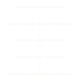
The earlier analytic steps remain input here. Locality supplies a quasi-local observable algebra and controlled dynamics. Positivity and the C*-norm make functional calculus meaningful. A thermodynamic gap supplies the physical phase condition. The present question is what can be transported from a microscopic system to an effective or homotopical target, and whether that transport can be reversed.
The three arrows
We insist on the following factorization:


Here is a low-energy or spectral-reduction map. The map extracts a stable invariant. The dashed map is a realization problem. It is not a formal inverse of .
Definition 1 (Microscopic-to-low-energy comparison). A microscopic-to-low-energy comparison consists of a domain , a target category , and a rule together with a stated limit, approximation, or functional-calculus theorem that controls the rule.
Definition 2 (Invariant extraction). An invariant extraction is a map defined after fixing dimension, symmetry, stabilization, and equivalence. It is an equivalence only if faithfulness, fullness, and essential surjectivity are separately proved.
Definition 3 (Microscopic realization). A realization of is an explicit local or uniformly almost-local interaction, symmetry action, ground-state convention, and system-size-independent gap witness whose comparison class is .
The definitions prevent a common reversal error. The existence of an invariant map does not provide a microscopic model for every target class. Agreement of invariants does not imply a microscopic gapped path unless a completeness theorem has been proved in the chosen domain.
Contributions
The paper makes six claims of different strength.
We prove a controlled functional-calculus theorem for compact families of bounded free-fermion Hamiltonians with a common Fermi gap.
We define a relative operator K-class with respect to a chosen reference Hamiltonian and prove homotopy invariance and stacking additivity.
We give a precise retention and loss table for spectral flattening. Positive energy rescaling supplies a simple nonfaithfulness proof.
We extend the controlled construction to covariant disordered one-particle systems represented in , under a genuine C*-spectral gap.
We compute the SSH transition charge on a linking circle and prove that a staggered mass provides a gapped symmetry-breaking detour.
We use the BDI interaction reduction to show why the free result has a sharp domain boundary.
The paper does not claim a general microscopic/EFT equivalence. It also does not claim that every bordism or homotopy class has a local gapped lattice representative.
Status vocabulary
Every substantive result is assigned one of the following labels.
| Label | Meaning |
|---|---|
| established | A cited theorem or standard construction under the assumptions displayed here. |
| proposed | A definition or condensed organization introduced by this program. |
| conjectural | A precise assertion for which this paper gives no proof. |
| open | No proof or counterexample is known in the stated scope. |
| obstructed | A theorem or explicit counterexample rules out the claim as stated. |
The functional-calculus statements below are established. The condensed packaging is proposed. A general lattice/EFT equivalence is open. An unchanged extension of free K-theory to all interacting BDI phases is obstructed.
Domains, targets, and equivalences
Microscopic quadratic systems
Let be a countable metric lattice and let be the one-particle Hilbert space. In the simplest translation-invariant case, A finite-range one-particle Hamiltonian is a bounded self-adjoint operator whose matrix elements vanish beyond a fixed lattice distance. Exponential or summable decay gives broader controlled classes.
After Fourier transform, a translation-invariant finite-range Hamiltonian is a matrix-valued trigonometric polynomial More generally, one works with a self-adjoint element of a unital C*-algebra encoding position, covariance, disorder, or symmetry.
Definition 4 (Controlled free-fermion datum). A controlled free-fermion datum is a tuple where is a specified real, complex, graded, or twisted C*-algebra, , is a Fermi level, records the symmetry constraints, and is a reference datum of the same type. The datum is spectrally gapped when
We set after replacing by . The algebra and the representation class are part of the problem. Changing them can change the relevant K-group.
Interacting lattice systems
An interacting microscopic system is not generally described by a bounded element . It is described by an interaction finite-volume Hamiltonians, and thermodynamic dynamics. The formal infinite sum of all need not converge in the quasi-local algebra.
This distinction matters for spectral flattening. Continuous functional calculus applies directly to a bounded self-adjoint element of a C*-algebra. It does not turn an extensive many-body Hamiltonian into a bounded quasi-local observable. Many-body phase equivalence instead uses a uniform finite-volume or bulk gap, quasi-adiabatic continuation, and stabilization by atomic systems.
Warning 5 (Domain boundary). The theorem in section 3 concerns bounded one-particle Hamiltonians or bounded C*-algebra representatives. It is not a spectral-flattening theorem for an arbitrary interacting infinite-volume Hamiltonian.
What counts as an effective theory
The term effective field theory will be used in a restricted way. An effective description records fields, symmetries, couplings, and a regime of momenta or energies in which its correlation functions approximate those of a microscopic model to a stated accuracy. A topological field theory is a still coarser target, usually intended to retain only long-distance invertible response or defect data.
Definition 6 (Controlled effective description). For a microscopic datum , a controlled effective description consists of a scale , an effective action or Hamiltonian , observables , and an error statement for a specified class of observables, with in a specified limit.
Spectral flattening is not such an approximation. It is a homotopy inside the space of gapped bounded operators. It preserves a stable topological class while deliberately destroying the energy scale.
An equivalence audit
Any claimed comparison must answer more than whether a map can be written. We use the following audit throughout.
| Question | Required datum | Failure mode |
|---|---|---|
| Question | Required datum | Failure mode |
| Construction | A defined map on a stated domain | Formal analogy with no map |
| Homotopy invariance | A chosen path topology and gap condition | Gap closes along the path |
| Faithfulness | Distinct inputs remain distinct | Flattening forgets energy scales |
| Fullness | Target morphisms lift to microscopic morphisms | EFT deformation has no lattice lift |
| Essential surjectivity | Every target object has a preimage | Abstract class lacks a local model |
| Stacking | Direct sum or tensor product is respected | Stabilization conventions disagree |
| Symmetry | Real, graded, or twisted structure is retained | Forgetting symmetry opens a detour |
| Boundaries and defects | Boundary conditions enter the category | Bulk class omits boundary choices |
| Interactions | Domain is closed under allowed interactions | Free classification collapses |
| Uniform gap | One lower bound controls the family | Pointwise gaps approach zero |
Calling a comparison an equivalence requires affirmative answers in the chosen category. The controlled free-fermion map below proves construction, gapped-homotopy invariance, and stacking compatibility. It is intentionally not faithful to microscopic spectra.
Functional calculus and the controlled K-class
A common spectral gap
Let be compact Hausdorff and a unital complex C*-algebra. Write An element is equivalently a norm-continuous family .
Definition 7 (Uniform Fermi gap). A self-adjoint family has a uniform Fermi gap when for every .
Because is compact and is norm-continuous, pointwise invertibility is enough to produce some common positive gap. We state the quantitative constant because later parameter objects need not be compact, and because estimates depend on it.
Lemma 8 (Inverse and gap). For self-adjoint in a unital C*-algebra, the following are equivalent:
;
is invertible;
there is with .
For an invertible self-adjoint ,
Proof. The equivalence of the first two statements is the definition of the spectrum. The spectrum is compact, so exclusion of zero is equivalent to a positive distance from zero. For a normal element, continuous functional calculus gives which proves the last identity. ◻
Spectral flattening
Define the sign function on by It is continuous on the spectrum of any invertible self-adjoint element.
Theorem 9 (Controlled spectral flattening). Let be compact Hausdorff, let be a unital complex C*-algebra, and let have a uniform Fermi gap. Set Then:
and ;
;
evaluation commutes with flattening, and ;
the path remains invertible and preserves the positive and negative spectral subspaces.
Proof. Continuous functional calculus in defines . The scalar identities and on imply and . The projection identities for follow by direct algebra.
Every evaluation map is a unital star-homomorphism. Functoriality of continuous functional calculus gives part (c).
For , the scalar homotopy is If , then . If , then . Thus zero never enters the spectral image. Functional calculus identifies and proves part (d). ◻
Remark 10. The theorem is sometimes described as replacing all occupied energies by and all empty energies by . That description is correct only after the Fermi level and occupied convention are fixed.
Relative operator K-theory
The projection determines a class Following the difference-group viewpoint emphasized by Thiang [Thiang2016], we compare it with a reference system.
Definition 11 (Relative difference class). Let and be uniformly gapped self-adjoint elements of matrix algebras over , with all required symmetry data fixed. Their relative class is
The word relative here refers to a difference from a reference phase. It should not be confused with the relative group of a topological pair, which appears in the transition calculation later.
Proposition 12 (Gapped-homotopy invariance). Suppose is a norm-continuous path of self-adjoint elements in and one satisfies for every . Then is a norm-continuous path of projections and Consequently is constant in .
Proof. Regard the family as one self-adjoint element The common gap makes invertible. Theorem 3.3 gives a projection . Evaluation at yields . Thus the endpoints are homotopic projections and define the same K-class. ◻
Proposition 13 (Stacking additivity). For two controlled data and references over the same parameter space,
Proof. Functional calculus respects block direct sums, so Addition in is defined by block direct sum. Subtracting the corresponding reference identity gives the formula. ◻
Chiral symmetry and the odd class
Suppose a grading satisfies . Functional calculus preserves this oddness: .
Proposition 14 (Off-diagonal unitary). Assume the two graded summands have equal stabilized size. Then the flattened operator has the form for a unitary over . The chiral stable class is , or the relative difference after choosing a reference.
Proof. Oddness forces the diagonal blocks of to vanish. Self-adjointness identifies the upper-right block with the adjoint of the lower-left block. The identity then gives . The standard unitary picture of supplies the class. ◻
Real symmetries and particle-hole structures require the appropriate real or graded K-group. The complex formula must not be reused after discarding those structures. Kitaev’s periodic table [Kitaev2009] and the operator-algebraic treatment of Thiang [Thiang2016] explain these symmetry-sensitive targets.
Naturality in the parameter space
Let be continuous between compact Hausdorff spaces. Pullback gives a star-homomorphism
Proposition 15 (Parameter naturality). Under the assumptions of theorem 3.3,
Proof. The first identity is functoriality of continuous functional calculus under the star-homomorphism . The induced map on is additive and sends differences to differences, which proves the second identity. ◻
This naturality is the reliable part of the condensed interpretation. For a representable condensed parameter object , one evaluates the family on a compact or profinite test space and pulls back along maps of tests. Extending the construction to arbitrary condensed anima requires a sheaf or stack model of the Hamiltonian domain and is proposed, not proved by the elementary theorem above.
The information-loss contract
What the class retains
Within the controlled domain, spectral flattening retains the following stable data.
It retains the occupied versus empty grading determined by the chosen Fermi level.
It retains the connected component of the gapped self-adjoint operator in the stabilized topology.
It retains symmetry constraints that were built into the real, graded, or twisted target algebra.
It retains the direct-sum law represented by addition in K-theory.
Through pairings with cyclic cocycles or geometric cycles, it may retain quantized response coefficients under the additional hypotheses of those index theorems [Bellissard1994, ProdanSchulzBaldes2016].
The last item is not automatic from the abstract K-class alone. One must supply the pairing, regularity algebra, trace, and covariance data.
What the class forgets
The same map forgets several physically meaningful quantities.
| Discarded datum | Reason |
|---|---|
| Gap magnitude | Every nonzero eigenvalue is moved to or . |
| Dispersion | The dependence of energy magnitude on momentum disappears. |
| Fermi velocity | Positive rescaling and nonlinear deformation leave the sign unchanged. |
| Correlation length | It is not determined by a stable projection class. |
| Lieb-Robinson constants | They belong to the microscopic interaction and metric. |
| Coupling values | Many different couplings flatten to the same involution. |
| Finite-band unstable data | Stabilization allows addition of trivial bands. |
| Boundary convention | A bulk K-class alone does not choose an edge termination. |
| Interaction vertices | They lie outside the quadratic one-particle datum. |
Proposition 16 (Positive rescaling is invisible). Let be an invertible self-adjoint element of a unital C*-algebra and let . Then If , the gap magnitude is multiplied by . Thus spectral flattening is not faithful to microscopic energy scales.
Proof. On , because is positive. Functional calculus gives the first two identities. The spectrum scales by , so ◻
This one-line counterexample is enough to rule out any claim that the flattened K-class reconstructs the microscopic Hamiltonian.
Example 17 (Trivial-band stabilization). Let be gapped and let . Then represent the same reduced stable phase after the added occupied and empty atomic bands are included in the reference convention. The second system has two more bands and a new energy scale. Stable classification is designed to forget that difference.
A contract, not a reconstruction theorem
We summarize the controlled map as Its contract is:
| Clause | Content |
|---|---|
| Domain | Bounded quadratic data in a fixed C*-algebra with a Fermi gap. |
| Equivalence | Norm-continuous, symmetry-preserving gapped homotopy plus stabilization. |
| Output | A relative class in the appropriate operator K-group. |
| Guaranteed | Naturality, homotopy invariance, and stacking additivity. |
| Not guaranteed | Spectrum, dynamics, locality constants, EFT limit, or interacting completeness. |
| Inverse | No inverse is supplied. |
This contract matches the formal Lean representation
TopologicalPhases.Observables.
That library records an Aoki comparison provider and C*-conditions without pretending to prove the analytic theorem inside Lean’s standard library.
Low-energy theory is a separate map
Linearization near a crossing
Suppose a Bloch Hamiltonian depends smoothly on momentum and a mass parameter . Near an isolated crossing , one may have where the satisfy suitable Clifford relations. The first-order term is a Dirac Hamiltonian. Any scalar term proportional to the identity has already been removed by the Fermi-level convention before the crossing subspace is expanded.
Proposition 18 (Controlled local linearization). Let be twice continuously differentiable in a neighborhood of and suppose after restriction to a fixed finite crossing subspace. Then Taylor’s theorem gives with on a sufficiently small neighborhood.
Proof. This is Taylor’s theorem for maps from a finite-dimensional parameter space to the finite-dimensional normed vector space of matrices. The bound follows from a uniform bound on the second derivative on a compact neighborhood. ◻
The proposition controls a local matrix approximation. It does not prove convergence of an interacting lattice theory to a relativistic quantum field theory. Even in the quadratic setting, the crossing subspace, momentum window, symmetry action, and neglected bands must be specified.
Scaling limits require more data
A genuine microscopic-to-EFT theorem would need at least:
a sequence of lattice spacings or energy cutoffs;
a renormalization prescription for fields and couplings;
convergence of a stated class of correlation functions or operator algebras;
control of irrelevant operators in the chosen topology;
a proof that the microscopic symmetry and anomaly data descend;
treatment of boundaries and defects if the target theory includes them.
Condensed mathematics can organize the parameter object on which such data vary. It does not supply any of these estimates.
Warning 19 (Flattening is not renormalization). The homotopy acts on all energies in a gapped bounded operator. Renormalization integrates out or rescales degrees of freedom relative to an energy or length scale. The two maps can lead to related topological data, but they are not the same construction.
Many-to-one behavior of effective descriptions
Two lattice Hamiltonians can share the same linear Dirac term while differing in quadratic dispersion, remote bands, and short-distance interactions. For example, adding does not change the first-order Dirac operator but changes the ultraviolet spectrum. Likewise, adding a high-energy atomic band changes the microscopic Hilbert space without changing the low-energy crossing.
Thus is generally many-to-one even before applying . This is expected behavior for an effective theory. It blocks reconstruction unless extra ultraviolet data are retained.
From EFT data to stable classes
Kitaev’s free-fermion table [Kitaev2009] and related tenfold-way constructions [Schnyder2008, Ryu2010] extract stable classes after fixing dimension and symmetry. Teo and Kane extend the controlled free classification to defect families [TeoKane2010]. These are strong results in their stated free-fermion domains.
Freed and Hopkins classify deformation classes of reflection-positive invertible extended field theories using stable homotopy and bordism data [FreedHopkins2021]. Their application to lattice phases assumes the existence and validity of low-energy effective-field-theory approximations. The bordism calculation is not, by itself, a theorem producing a local lattice Hamiltonian.
Remark 20 (Dimension convention). Spatial lattice dimension is denoted . Spacetime dimension is . Bordism classifications are usually indexed by , while Bloch Hamiltonians are indexed by . The two indices must not be silently identified.
Disorder and the covariant observable algebra
A profinite disorder hull
Let be a finite set of local labels and set With the product topology, is compact, Hausdorff, and profinite. The translation action shifts a configuration.
The covariant bulk algebra is Because is amenable, full and reduced crossed products agree. A magnetic field may require a twisted crossed product. This noncommutative Brillouin-zone viewpoint underlies rigorous treatments of disordered topological phases and the quantum Hall effect [Bellissard1994, ProdanSchulzBaldes2016].
Finite-range covariant Hamiltonians
A finite-range covariant one-particle Hamiltonian can be written schematically as where the implement translations. The coefficients satisfy the adjoint relations that make . The finite sum is an element of .
Theorem 21 (Disordered Fermi projection). Let and suppose Then belongs to and defines . Norm-continuous paths that remain invertible preserve this class.
Proof. Apply continuous functional calculus in the crossed-product C*-algebra. The homotopy statement is theorem 3.6 with a one-point parameter space. ◻
This result justifies the disorder algebra where a genuine spectral gap is present. It does not claim that every configuration has a gap merely because is compact. The gap is a spectral property of the crossed-product element.
Mobility gaps are not spectral gaps
Disordered topological phases can remain quantized when the Fermi energy lies in a localized regime even though it belongs to the spectrum. That situation requires mobility-gap hypotheses, Sobolev or localization algebras, trace estimates, and index pairings. The discontinuous characteristic function is then handled in a more refined regularity framework.
Warning 22. Theorem 6.1 assumes a C*-spectral gap. It must not be cited as a mobility-gap theorem. The latter theory is deeper and has different hypotheses [Bellissard1994, ProdanSchulzBaldes2016].
What profinite approximation does and does not prove
Locally constant functions that factor through finite clopen quotients are sup-norm dense in . This gives finite-resolution approximations to coefficient functions. It does not imply that every K-class, spectral gap, or response coefficient is determined by one finite quotient.
The safe condensed statement is functorial: the profinite space is a legitimate test object, covariant families pull back along maps of disorder spaces, and their K-classes are natural when the analytic hypotheses survive pullback. The sheaf condition does not manufacture the crossed-product spectrum or its gap.
The SSH model as a complete controlled example
Bloch Hamiltonian and spectrum
The spinless SSH Bloch Hamiltonian is It anticommutes with the chiral operator . Writing the energies are The model descends from the dimerized chain introduced by Su, Schrieffer, and Heeger [SSH1979].
Proposition 23 (SSH gap). For real , the distance from zero to the spectrum is The separation between the occupied and empty bands is The gap closes exactly when .
Proof. The squared positive energy is Its minimum over is Taking square roots gives the half-gap. The two bands lie symmetrically about zero, so their separation is twice that number. ◻
Flattening and winding
When the model is gapped, define The flattened Hamiltonian is
Proposition 24 (SSH winding). Assume and . With the convention ,
Proof. The curve is a circle of radius centered at the real number . Multiplication by a nonzero real rotates the parametrized circle by zero or but does not reverse its orientation. The circle winds once counterclockwise around zero precisely when its center lies inside its radius. Otherwise it has winding zero. ◻
Choose a trivial reference with . Then the relative AIII class of a topological sample is one. This is a concrete instance of the relative construction in theorem 3.8.
The gapless discriminant
The global coupling discriminant is Near the branch and momentum , write Then The combined momentum-mass plane is essential. Looking only at the coupling line misses the linking circle around the isolated degeneracy in .
Proposition 25 (Local SSH transition charge). Fix and orient the small linking circle by To leading order, Its degree is . Reversing the circle orientation changes the sign. The absolute charge is one and equals the magnitude of the winding jump.
Proof. Substitution gives Normalization removes . The map has degree . The higher-order term is uniformly smaller than on a sufficiently small circle, so it can be removed by a homotopy that avoids zero. ◻
Topologically, the normalized map defines a class in The connecting morphism for the pair sends it to This is the elementary model for a relative transition charge. Teo and Kane’s free-fermion defect theory gives the broader controlled precedent [TeoKane2010].
A symmetry-breaking detour
Add a staggered sublattice potential The Hamiltonian becomes For , it no longer anticommutes with .
Theorem 26 (Gapped detour after forgetting chiral symmetry). Fix and . For , set The endpoint at is the chiral trivial phase and the endpoint at is the chiral topological phase. Along the full path, the occupied-empty band separation is exactly . The interior breaks chiral symmetry.
Proof. Since , both and are positive. The minimum positive energy is Thus the full band separation is . At the endpoints . For , and the chiral anticommutation relation fails. ◻
The theorem shows that the SSH charge is relative to the AIII symmetry problem. If the symmetry is removed from the category, the two endpoints are gapped-homotopic. This is not a failure of the AIII invariant. It is a reminder that symmetry is part of its domain.
Executable finite checks
The accompanying Haskell program implements the exact two-band formulas. Its checks include:
| Check | Scope |
|---|---|
| SSH spectrum and analytic gap | Finite Bloch matrices |
| Normalized flattened vector | Sampled momenta away from the discriminant |
| Analytic and numerical winding | AIII two-band family |
| Relative winding difference | Chosen trivial reference |
| Local linking degree | The circle |
| Symmetry-breaking detour | A sampled semicircle with exact gap formula |
| Information-loss contract | Nonempty, pairwise-disjoint information categories |
| Three-arrow audit | Distinct typed statuses |
The code compiles with strict warnings and exits nonzero if a check fails. It is not evidence for a general thermodynamic limit.
Interactions: the BDI boundary
The free integer invariant
Class BDI describes one-dimensional free fermions with particle-hole symmetry, time-reversal symmetry squaring to , and their product chiral symmetry. In the stable free classification, the phase index is an integer. Stacking adds the integers.
This statement is different from the complex AIII SSH invariant, even though both use winding in simple matrix representatives. The real symmetry structure changes the classification problem.
Fidkowski-Kitaev reduction
Fidkowski and Kitaev constructed a symmetry-preserving interacting path that connects free BDI phases whose integer labels differ by eight [FidkowskiKitaev2009]. They later proved that the eight residue classes are distinct and exhaustive for the specified one-dimensional interacting fermionic problem [FidkowskiKitaev2011].
Theorem 27 (BDI interaction reduction, cited). Within the one-dimensional BDI setting of [FidkowskiKitaev2009, FidkowskiKitaev2011], the stable free index descends under symmetry-preserving interactions to In particular, eight copies of the generating free chain admit a gapped interacting deformation to the trivial phase.
Source-based proof sketch. Fidkowski and Kitaev identify the boundary Majorana degrees of freedom and construct quartic interactions that gap eight modes without breaking the BDI symmetry. Their explicit interacting path avoids the free critical locus while remaining gapped. The matrix-product-state and central-extension analysis distinguishes the eight remaining classes and proves exhaustion. The full proof is contained in the cited papers; it is not reproduced here. ◻
What the reduction proves
The reduction proves that the free classification is not a complete invariant of the larger interacting category. It does not invalidate the free functional-calculus theorem. That theorem remains correct on its quadratic domain.
The categorical picture is a quotient-like comparison after the class of allowed paths is enlarged to include interactions. The kernel is not visible within free gapped homotopy.
Corollary 28 (No unchanged universal extension). There is no classification of all interacting one-dimensional BDI phases by the free integer invariant that simultaneously agrees with free stacking and identifies phases connected by the Fidkowski-Kitaev interacting paths.
Proof. The free invariant assigns different integers to phases whose labels differ by eight. The cited interacting path declares those phases equivalent. Any invariant of interacting phase equivalence must take equal values on the two endpoints. Therefore the free integer cannot descend unchanged. ◻
This gives a direct counterexample to the identification of microscopic phases with free K-theory.
Realization is not the inverse map
Stable free representatives
In controlled free-fermion problems, Bott periodicity and Clifford-module constructions often provide representatives for stable K-classes [Kitaev2009, Thiang2016]. Lattice Dirac models can realize many table entries after fixing a symmetry class and allowing stabilization.
Even there, one must distinguish:
a continuous family of finite matrices on a Brillouin torus;
a finite-range or rapidly decaying real-space Hamiltonian;
a chosen boundary termination;
a material realization with fixed orbital constraints.
A homotopy class of maps may have a continuous representative whose Fourier coefficients decay but are not finite range. Approximation can often recover finite range while preserving a positive gap, but the approximation theorem and symmetry constraints must be stated.
Interacting and bordism classes
For an abstract invertible field-theory or bordism class, a microscopic realization needs more:
local degrees of freedom and an on-site or spatial symmetry action;
a uniformly local or almost-local interaction;
a ground-state and boundary convention;
a gap uniform in system size;
a computation identifying the low-energy or response class;
an inverse under stacking if invertibility is claimed.
The bordism group does not package these witnesses. It classifies field-theoretic deformation data under its own axioms. Freed and Hopkins explicitly frame the lattice application through an EFT assumption [FreedHopkins2021].
Definition 29 (Realization status). For a candidate class , assign one of the following statuses:
realized: an explicit local interaction, symmetry, uniform gap theorem, and comparison computation are known;
candidate: a model exists, but one of those checks is incomplete;
open: no realization or obstruction theorem is known;
obstructed: a theorem rules out realization under the stated microscopic rules.
Absence of a known model means open, not obstructed.
Why surjectivity is hard
Essential surjectivity of a realization map would require every abstract class to admit a microscopic witness. Three independent obstructions can intervene.
First, the abstract target may assume relativistic locality or full extension to defects that a lattice construction has not supplied. Second, anomaly constraints may force a boundary interpretation rather than an autonomous lattice bulk in the stated dimension. Third, a formal phase label may have no known system-size-independent gap proof for its proposed Hamiltonian.
These are mathematical requirements, not matters of terminology.
Why injectivity is hard
Injectivity would say that two microscopic phases with the same abstract class are connected by an allowed stabilized gapped path. The target class may omit crystalline data, noninvertible excitations, boundary conditions, or unstable finite-band information. If any omitted datum is retained by the microscopic equivalence, injectivity fails.
The BDI reduction shows the opposite possibility as well. Enlarging the microscopic path category can identify free classes that were distinct before interactions were allowed. The answer depends on the domain and its morphisms.
A condensed-mathematics formulation
Representable parameter objects
For a compactly generated space , write on profinite test spaces . The precise full-faithfulness statement uses the compact-generation and cardinal conventions of condensed mathematics [Scholze2026].
A compact parameter family of controlled Hamiltonians is an element The uniformly gapped locus consists of those for which one lower bound works on all of . Theorem 3.3 gives a natural map
Proposition 30 (Descent at the C*-algebra level). Let be a finite jointly surjective family of profinite spaces. Then is an isomorphism of C*-algebras. Compatible flattened projections glue uniquely.
Proof. Continuous functions glue uniquely across a finite jointly surjective compact Hausdorff cover because the induced disjoint-union map is a quotient map. Operations, involution, and the sup norm are pointwise. The projection equation is also pointwise, so compatible local projections glue to a projection. ◻
This is an exact statement about representable profinite tests. It does not prove that the spectral gap itself descends from arbitrary local gap constants unless the constants have a common positive lower bound.
The proposed comparison diagram
The controlled map and the broader comparison program are displayed as two separate chains:


The first arrow is the theorem proved in the controlled free sector. In the second chain, is solid only on the specified reflection-positive invertible-EFT domain classified by Freed and Hopkins. The low-energy map and the realization map require separate comparison and realization theorems. No map and no commutative comparison square are claimed here.
Solidification is a K-theory bridge
Aoki proves that solidification of algebraic K-theory recovers connective topological K-theory for real and complex Banach algebras, with the stated connective and Bott-periodic qualifications [Aoki2024]. This supplies a genuine condensed-to-operator K-theory bridge.
It does not reconstruct the C*-norm, positive cone, state space, or microscopic interaction. It also does not prove that every operator K-class is a physical phase. The bridge is at the level of K-theory after the Banach algebra is already given.
Status ledger and formal interfaces
Claim ledger
| Status | Claim | Hypotheses or source |
|---|---|---|
| Status | Claim | Hypotheses or source |
| established | Continuous functional calculus produces the flattened involution and Fermi projection. | Bounded self-adjoint C*-element with a spectral gap. |
| established | Gapped norm-continuous paths preserve the K-class. | Common gap and fixed algebra/symmetry. |
| established | The relative class is additive under block direct sum. | Fixed reference and stabilization convention. |
| established | The SSH winding is one inside the coupling circle and zero outside. | Gapped chiral two-band model. |
| established | The local SSH linking charge has magnitude one. | Fixed orientation near the isolated crossing. |
| established | A staggered mass opens a gapped detour. | Chiral symmetry is not required along the path. |
| established | BDI interactions reduce the free integer to eight classes. | Fidkowski-Kitaev one-dimensional symmetry setting. |
| established | A crossed-product Fermi projection gives a K-class. | Covariant bounded Hamiltonian with C*-spectral gap. |
| proposed | These maps assemble into a condensed Hamiltonian-stack comparison. | Representable tests are controlled; general stack construction remains. |
| open | General interacting microscopic systems are equivalent to an EFT stack. | No theorem in this scope. |
| open | Every abstract invertible bordism class has a local gapped lattice representative. | Requires explicit realization and uniform gap. |
| obstructed | Free K-theory classifies all interacting BDI phases without modification. | Counterexample from the eightfold reduction. |
Lean representation
The reviewed Lean foundation intentionally represents theorem interfaces, not deep analytic proofs. The declarations relevant here include:
ClaimStatusandProvenancefor the status ledger;FiniteVolumeGapWitnessfor an explicit common lower bound;ObjectwiseInvolutionandObjectwiseCStarNormConditionsfor operator-algebraic input;StackingandPhaseEquivalencefor the stable phase interface;AokiConnectiveComparisonInterfacefor the imported solidification theorem.
No Lean declaration in that foundation asserts a Lieb-Robinson estimate, thermodynamic limit, or Aoki comparison without a provider. The library builds without user axioms.
Haskell representation
The Haskell directory src/microscopic-effective-theories/ contains four modules.
| Module | Role |
|---|---|
Core.hs | SSH spectrum, gap, flattening, winding, detour, contracts |
Properties.hs | Deterministic behavioral properties |
Proofs.hs | Finite equational and numerical checks |
Main.hs | Demonstrations, checks, and nonzero failure exit |
All top-level bindings have explicit type signatures and each module has an explicit export list. The strict compiler flags are The program uses no claim stronger than its finite computations.
Limitations and open comparison problems
Interacting spectral flattening
A general interacting infinite-volume system has no bounded one-particle Hamiltonian to which this construction can be applied. One can flatten finite-volume matrices, but the resulting operator may be highly nonlocal and need not converge to a quasi-local thermodynamic object. Spectral flow is the more appropriate interacting tool, provided a uniform gap and locality estimates have already been proved.
An open comparison problem is to relate interacting spectral-flow classes to operator-algebraic or generalized cohomology invariants without discarding the relevant higher defects.
Noninvertible topological order
A spectrum of invertible phases cannot classify general noninvertible topological order. Anyons, fusion, braiding, and higher defect categories require richer targets. Two systems can share an invertible response class while having different noninvertible excitation data.
The paper therefore restricts its bordism discussion to invertible sectors.
Boundaries
Bulk K-theory can pair with boundary maps and produce bulk-boundary correspondences under controlled hypotheses [ProdanSchulzBaldes2016, TeoKane2010]. A bulk class alone does not specify a boundary Hamiltonian, termination, or symmetry-breaking boundary condition. Any claimed microscopic/EFT equivalence with boundaries must include those objects and their morphisms.
Crystalline and spatial symmetries
Spatial symmetries are not ordinary on-site internal symmetries. Their action on momentum, position, disorder, and defects changes the target K-theory or equivariant homotopy theory. A comparison that forgets the spatial action can merge distinct crystalline phases.
The present paper treats symmetry abstractly through a fixed C*-algebraic structure and does not claim a complete crystalline classification.
Mobility-gap extension
A mobility-gap extension matters for disordered systems. It requires localization estimates that ensure the Fermi projection belongs to an algebra on which index pairings remain defined. Developing that extension in condensed families would require uniform localization control across the parameter object. Compactness or profiniteness alone does not provide it.
Realization tests
A useful next step is a machine-readable realization registry. Each row would record:
the abstract class and symmetry type;
an explicit microscopic interaction;
a locality certificate;
a uniform gap theorem;
a class computation;
the status realized, candidate, open, or obstructed.
Such a registry would expose which part of the inverse problem is missing for each example.
Discussion
The controlled theorem starts only after a C*-algebra has been chosen and the Hamiltonian is bounded and self-adjoint, the Fermi level is uniformly isolated, and the symmetry and reference are fixed. Under those assumptions, functional calculus gives a stable class with clean naturality properties.
The loss is built into stable K-theory, which forgets deformations and added trivial bands. Describing that quotient as a reconstruction of the microscopic system would be incorrect.
The SSH calculation makes both sides visible. Within AIII symmetry, the winding jump forces a gap closing and the linking circle has charge one in magnitude. Once the staggered mass is permitted, the detour keeps a constant gap. The category changed, so the classification changed.
The BDI example makes the same point at the interaction boundary. Allowing quartic interactions enlarges the path space and identifies every eighth free phase. No amount of categorical packaging removes that physical fact.
Condensed mathematics enters most cleanly through parameter functoriality and the treatment of profinite disorder spaces. It places continuous families, inverse limits, and descent in one formal setting. Its contribution is organizational and homological. The analytic inputs remain locality, positivity, spectral control, and the existence of comparison maps.
Conclusion
There is a rigorous bridge from a controlled free-fermion Hamiltonian to a relative operator K-class: The bridge is natural in compact parameter spaces, invariant under uniformly gapped norm-continuous homotopy, and additive under stacking. For chiral systems it has the corresponding odd-unitary form. For spectrally gapped covariant disorder models it lives in the K-theory of a crossed product.
This bridge is not an equivalence between microscopic lattice systems and effective field theories. It forgets energy scales and much of the ultraviolet model. It does not include general interactions. It has no automatic inverse realization map.
The correct research program therefore keeps the three arrows separate. One proves a low-energy limit where possible, extracts an invariant under fixed hypotheses, and treats microscopic realization as its own theorem or open problem. The SSH transition and the BDI interaction reduction show why those distinctions are physically necessary.
Functional-calculus details
Continuity of the sign map on a gapped set
Fix and . On the compact set the sign function is continuous. By the Stone-Weierstrass theorem, polynomials can approximate it uniformly on . If is self-adjoint with , then is the norm limit of the same polynomials in .
For a norm-continuous family with a common gap and a common norm bound, the polynomial approximants are uniformly continuous in the family parameter. Their uniform limit is norm-continuous. This gives an elementary route to the continuity assertion in theorem 3.6.
A resolvent formula
The negative spectral projection can also be written as a Riesz projection. Choose a contour enclosing the negative spectrum and excluding the positive spectrum. Then If is close enough to , the same contour lies in the resolvent set of . The resolvent identity gives norm continuity of the projection.
This formula also displays the role of the gap. As the contour approaches the spectrum, the resolvent norm grows and uniform control is lost.
Symmetry functoriality
Suppose an automorphism or anti-automorphism encodes a symmetry and obeys a relation such as Functional calculus transports the corresponding relation to because the sign function is real and odd. The target K-group must still remember whether is linear, antilinear, grading-preserving, or grading-reversing.
Difference classes and references
Why a reference is useful
The Grothendieck group of projections contains formal differences. Physically, choosing identifies which atomic or vacuum configuration counts as zero. The class then measures an obstruction between two gapped data rather than assigning an absolute label to one Hamiltonian.
Thiang’s formulation makes this relative viewpoint explicit [Thiang2016]. It avoids suggesting that the abstract group element contains a preferred microscopic representative.
Cocycle law
For three controlled systems in the same target, where The formula is immediate by cancellation in the abelian group. It is checked on finite SSH representatives by the Haskell program.
Reference changes
If the reference is changed from to , then Thus absolute coordinates change by a constant translation. Differences between two physical systems do not depend on that coordinate choice.
SSH conventions and numerical checks
Orientation
With the topological SSH winding is for . Near , the local coordinate is The positively oriented circle maps to and therefore has degree . There is no contradiction. The local charge and the phase jump use different boundary orientations. Only the orientation-adjusted equality, or equality in magnitude, is canonical.
Discrete winding computation
For nonzero samples with , the code computes The analytic gap check runs first, so division by zero is excluded. Set and . Since the code requires before summing principal phase increments. This sufficient sampling condition prevents a true increment from crossing the branch cut; an explicit runtime check rejects an increment of magnitude as well. The result then agrees with theorem 7.2.
The computation is a regression test for the implementation. It is not used as the proof of the analytic proposition.
Finite gap sampling
The executable proof check compares the closed formula with the minimum sampled band separation on a mesh that contains . The analytic derivation remains the proof. The mesh catches sign, factor-of-two, and convention mistakes in code.
Comparison checklist for later work
Before a future paper claims a microscopic/EFT equivalence, it should fill in the following record.
| Field | Required answer |
|---|---|
| Field | Required answer |
| Microscopic objects | Interactions, Hilbert spaces, symmetries, and boundary conventions. |
| Microscopic morphisms | Exact definition of gapped path, circuit, or quasi-local equivalence. |
| Effective objects | Fields, tangential structure, anomalies, and defect depth. |
| Effective morphisms | Deformation, natural equivalence, or bordism convention. |
| Limit | Scaling parameter and topology of convergence. |
| Uniformity | Bounds uniform in volume and external parameters. |
| Construction | Formula or theorem defining the forward map. |
| Invariance | Proof that microscopic equivalences map to effective equivalences. |
| Faithfulness | Proof or counterexample. |
| Fullness | Proof that effective morphisms lift. |
| Surjectivity | Realization theorem for every target class. |
| Stacking | Compatibility with direct sum or tensor product. |
| Symmetry | Preservation of internal, antiunitary, and spatial actions. |
| Boundary | Treatment of edges, defects, and anomaly inflow. |
| Lost data | Explicit list of ultraviolet information removed by the map. |
| Interaction boundary | Statement of which nonquadratic perturbations are admitted. |
Most known general comparisons fill only part of this record. That is still mathematically useful. The problem arises when a partial invariant-producing map is reported as a categorical equivalence.
99
K. Aoki, (Semi)topological K-theory via solidification, arXiv:2409.01462, 2024.
M. F. Atiyah, K-Theory, W. A. Benjamin, 1967.
J. Bellissard, A. van Elst, and H. Schulz-Baldes, The non-commutative geometry of the quantum Hall effect, Journal of Mathematical Physics 35 (1994), pages 5373 to 5451, doi:10.1063/1.530758.
B. Blackadar, K-Theory for Operator Algebras, second edition, Cambridge University Press, 1998.
P. Scholze, Lectures on Condensed Mathematics, arXiv:2605.03658, 2026.
L. Fidkowski and A. Kitaev, The effects of interactions on the topological classification of free fermion systems, Physical Review B 81 (2010), 134509, doi:10.1103/PhysRevB.81.134509.
L. Fidkowski and A. Kitaev, Topological phases of fermions in one dimension, Physical Review B 83 (2011), 075103, doi:10.1103/PhysRevB.83.075103.
D. S. Freed and M. J. Hopkins, Reflection positivity and invertible topological phases, Geometry & Topology 25 (2021), pages 1165 to 1330, doi:10.2140/gt.2021.25.1165.
A. Kitaev, Unpaired Majorana fermions in quantum wires, Physics-Uspekhi 44 (2001), pages 131 to 136, doi:10.1070/1063-7869/44/10S/S29.
A. Kitaev, Periodic table for topological insulators and superconductors, AIP Conference Proceedings 1134 (2009), pages 22 to 30, doi:10.1063/1.3149495.
E. Prodan and H. Schulz-Baldes, Bulk and Boundary Invariants for Complex Topological Insulators, Springer, 2016, doi:10.1007/978-3-319-29351-6.
S. Ryu, A. P. Schnyder, A. Furusaki, and A. W. W. Ludwig, Topological insulators and superconductors: tenfold way and dimensional hierarchy, New Journal of Physics 12 (2010), 065010, doi:10.1088/1367-2630/12/6/065010.
A. P. Schnyder, S. Ryu, A. Furusaki, and A. W. W. Ludwig, Classification of topological insulators and superconductors in three spatial dimensions, Physical Review B 78 (2008), 195125, doi:10.1103/PhysRevB.78.195125.
W. P. Su, J. R. Schrieffer, and A. J. Heeger, Solitons in polyacetylene, Physical Review Letters 42 (1979), pages 1698 to 1701, doi:10.1103/PhysRevLett.42.1698.
J. C. Y. Teo and C. L. Kane, Topological defects and gapless modes in insulators and superconductors, Physical Review B 82 (2010), 115120, doi:10.1103/PhysRevB.82.115120.
G. C. Thiang, On the K-theoretic classification of topological phases of matter, Annales Henri Poincare 17 (2016), pages 757 to 794, doi:10.1007/s00023-015-0418-9.