The Invertible Condensed Phase Spectrum Program

Five stages, not five equivalences

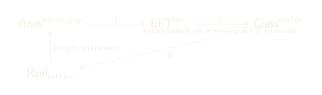
Write the proposed sequence as $$\begin{equation} \mathsf{Int}^{\mathrm{ub}}_{\mathcal F} \longrightarrow \mathfrak{Ham}_{\mathcal F} \longleftarrow \mathfrak{Gap}^{\mathrm{prop}}_{\mathcal F} \longrightarrow \mathfrak{Phase}^{\mathrm{st}}_{\mathcal F} \longrightarrow \mathit{IP}^{\mathrm{cond}}_{\mathcal F}. \tag{1} \end{equation}$$ The reverse arrow at the gapped stage is intentional: a gapped subobject, if it exists, includes into the Hamiltonian moduli object. A quantitative witness object maps to both. The prose sequence records a flow of construction; the categorical diagram records the variance correctly.

No arrow in equation (1) is declared an equivalence. The first packages analytic data. The second takes a propositional image. The third localizes and stabilizes. The fourth passes to stacking-invertible objects and then, conditionally, to a spectrum.

Spatial and spacetime grading

We use $$\begin{equation} d=\text{spatial dimension}, \qquad n=d+1=\text{spacetime dimension}. \tag{2} \end{equation}$$ Microscopic interactions and Kubota’s construction are graded by $d$. Field-theory tangential structures are graded by $n$. Any comparison must display the shift. Suppressing it can make two formulas look identical even when they classify different dimensional objects.

Scope

The target is the invertible sector. Intrinsic topological order with noninvertible excitations needs fusion, braiding, and defect categories that cannot be recovered from a spectrum of units. Crystalline symmetry, fermionic grading, and disorder may be included only after their actions are specified in the microscopic category. This paper describes interfaces for that work rather than claiming a complete classification.

An evidence order

Statuses do not form a simple scale from weak to strong. An obstructed implication can be known more firmly than a proposed construction. For validation purposes it is better to record provenance separately: $$\begin{equation} \text{claim}\quad+\quad\text{status}\quad+\quad \text{hypotheses}\quad+\quad\text{provider}. \tag{3} \end{equation}$$ A provider may be a theorem, an explicit calculation, a cited construction, or a named open comparison problem. The Haskell code mirrors equation (3); it never tries to infer truth from a status label.

Nonclaims fixed at the outset

The following statements are excluded.

1. A profinite parameter space does not imply a uniform locality bound.

2. Pointwise finite-volume gaps do not imply a thermodynamic gap.

3. A ring with involution is not automatically a C*-algebra.

4. A K-class does not reconstruct a Hamiltonian.

5. A low-energy field theory is not automatically equivalent to its microscopic lattice model.

6. Isomorphic homotopy groups do not identify spectra.

7. An abstract bordism class does not provide a microscopic realization.

8. A relative cohomology class is not automatically a measurable transition charge.

These exclusions are not philosophical caution. Each one corresponds to a missing hypothesis or a known loss of information.

Established locality output

This theorem is analytic input, not a consequence of condensed descent. A test object organizes the parameter dependence; it does not manufacture the common constant in equation (6).

Restriction and finite descent

For a map $f:T\to S$, restriction sends $\Phi$ to $f^*\Phi$. The same uniform locality bound remains valid. For a finite jointly surjective cover $S_i\to S$ of profinite spaces, compatible local coefficient functions glue because the disjoint union map is a quotient map. A common numerical bound also glues if it has been supplied on the entire finite cover, for example by taking the maximum of finitely many bounds.

This gives a controlled set-valued sheaf of interaction objects on the chosen finite-cover site. It does not yet give the higher moduli stack used later. Morphisms, automorphisms, and higher coherences still have to be defined.

Objectwise C*-algebraic control

For a compact Hausdorff parameter space $S$ and a C*-algebra $\mathcal A$, the continuous family algebra $$\begin{equation} C(S,\mathcal A) \end{equation}$$ is a C*-algebra with pointwise operations, involution, and norm $$\begin{equation} \|a\|=\sup_{s\in S}\|a(s)\|_{\mathcal A}. \end{equation}$$ Positivity is fiberwise: $$\begin{equation} a\ge0 \quad\Longleftrightarrow\quad a(s)\ge0\text{ for every }s\in S. \tag{10} \end{equation}$$ The C*-identity follows exactly: $$\begin{equation} \|a^*a\| = \sup_s\|a(s)^*a(s)\| = \sup_s\|a(s)\|^2 = \|a\|^2. \tag{11} \end{equation}$$

These statements solve the positivity and norm problem once the fixed C*-algebra $\mathcal A$ has been chosen. They do not construct that norm from bare algebraic multiplication and involution.

Finite-cover C*-descent

If $S_i\to S$ is a finite jointly surjective family of profinite spaces, then $$\begin{equation} C(S,\mathcal A) \cong \operatorname{Eq}\left( \prod_i C(S_i,\mathcal A) \rightrightarrows \prod_{i,j}C(S_i\times_S S_j,\mathcal A) \right) \tag{12} \end{equation}$$ as C*-algebras. The norm on a glued section is forced by the fiberwise supremum. Positivity and self-adjointness descend because they are tested fiberwise.

Finite clopen partitions give dense finite approximations to continuous functions on a profinite space. They do not imply that every continuous family factors exactly through a finite quotient. That stronger assertion would discard genuine continuous variation.

States are not pointwise state-valued maps

A state on $C(S,\mathcal A)$ contains a probability measure on $S$ together with conditional state data. In general, $$\begin{equation} \operatorname{State}(C(S,\mathcal A)) \ne C(S,\operatorname{State}(\mathcal A)). \tag{13} \end{equation}$$ The right side chooses one normalized state at every point. The left side can average over the parameter space. This distinction is relevant when a ground-state sector is part of a gap witness.

The proposed moduli stack

Let $\mathsf{CondTest}$ be a chosen site of condensed test objects. Its precise size, topology, and hypercompletion convention must be fixed. For each $S$, define a tentative category $\mathcal C_{\mathfrak{Ham}}(S)$ whose objects include:

1. a lattice or relaxed-lattice datum of spatial dimension $d$;

2. a continuous field of local finite-dimensional algebras;

3. a uniformly $F$-local self-adjoint interaction;

4. symmetry and grading data;

5. boundary and ground-state conventions when required.

Morphisms should record controlled changes of presentation, such as local unitary identifications, lattice refinements, or paths of interactions. The choice determines the eventual phase relation.

The word “provided” carries real content. Objectwise finite-cover descent does not automatically prove descent for path spaces, automorphism groups, spectral-flow providers, or variable lattices. The existence of equation (14) with all desired structures is Proposed.

Finite-volume and GNS witnesses

Fix a family of finite volumes $\Lambda_L$ and a prescribed low-energy sector of dimension $m_L$. A uniform finite-volume witness contains a number $\gamma>0$ and a threshold $L_0$ such that $$\begin{equation} E_{m_L+1}(H_{\Lambda_L,s})-E_{m_L}(H_{\Lambda_L,s}) \ge\gamma \tag{15} \end{equation}$$ for every $L\ge L_0$ and every parameter $s$.

An infinite-volume GNS witness instead chooses a ground state $\omega_s$, its GNS representation, and a positive generator $K_s$ of the implemented dynamics such that $$\begin{equation} \operatorname{Spec}(K_s)\cap(0,\gamma)=\varnothing \tag{16} \end{equation}$$ uniformly in $s$. Relating the two notions requires hypotheses on boundary conditions, ground-state sectors, and the thermodynamic limit. The paper does not treat them as definitionally equal.

Witnesses form a fibration of data

Let $W(S)$ denote the type of accepted gap witnesses over an $S$-family. Define $$\begin{equation} \mathfrak{Gap}^{\mathrm{wit}}_{\mathcal F}(S) = \{(H,w): H\in\mathfrak{Ham}_{\mathcal F}(S),\ w\in W_S(H)\}. \tag{17} \end{equation}$$ Forgetting the numerical and ground-state data gives $$\begin{equation} p_S:\mathfrak{Gap}^{\mathrm{wit}}_{\mathcal F}(S)\longrightarrow\mathfrak{Ham}_{\mathcal F}(S). \tag{18} \end{equation}$$

This is more than a set-theoretic nuisance. Loops in the space of witnesses can contain information about choices that should disappear from a phase label. Treating equation (18) as an inclusion would retain that information by mistake.

The propositional image

The qualitative predicate is obtained by truncating the existence of a witness: $$\begin{equation} \mathfrak{Gap}^{\mathrm{prop}}_{\mathcal F}(S) = \{H\in\mathfrak{Ham}_{\mathcal F}(S):\|\exists w\in W_S(H)\|\}. \tag{19} \end{equation}$$ Here the vertical bars denote propositional truncation. Equivalently, $\mathfrak{Gap}^{\mathrm{prop}}$ is the image of $p$ when the chosen category of condensed anima has pullback-stable image factorizations.

Descent can combine witnesses that already exist. It cannot infer a common positive lower bound from unrelated local or pointwise gaps. For a finite cover, finitely many compatible lower bounds have a positive minimum. For an infinite cover, the infimum can be zero.

Gap stability

The theorem begins with a uniform gap. It does not prove that a proposed path is gapped. Establishing the gap is often the hardest analytic task in a phase classification.

The path category

For a test object $S$, let $\mathcal C_{\mathrm{gap}}(S)$ be the proposed category whose objects are $S$-families in $\mathfrak{Gap}^{\mathrm{prop}}(S)$ and whose morphisms are controlled uniformly gapped interpolations, quasi-local automorphisms supplied by spectral flow, and specified changes of local presentation. Every morphism carries a provider showing that locality and the gap remain uniform over both $S$ and the interpolation parameter.

Let $W(S)$ be the class of morphisms declared to be phase equivalences. A calculus of fractions is not assumed automatically. The infinity-categorical localization $$\begin{equation} \mathcal C_{\mathrm{gap}}(S)[W(S)^{-1}] \tag{20} \end{equation}$$ exists abstractly in a sufficiently large ambient category, but size, descent, and compatibility with stacking must still be checked.

Stabilization

Choose a class $\mathsf{At}$ of atomic product-state systems. Stacking with an atomic ancilla gives transition functors $$\begin{equation} H\longmapsto H\boxtimes A, \qquad A\in\mathsf{At}. \end{equation}$$ The stabilized category is a filtered colimit only after maps between ancilla choices and their coherences have been specified. Formally, write $$\begin{equation} \mathcal C_{\mathrm{gap}}^{\mathrm{st}}(S) = \operatorname*{colim}_{A\in\mathsf{At}} \mathcal C_{\mathrm{gap}}(S)[W(S)^{-1}]. \tag{22} \end{equation}$$

Taking the core discards noninvertible categorical morphisms but retains all equivalences and their higher homotopies. It does not make every object invertible under stacking. That is a separate operation.

Why stabilization changes the question

Two finite-band Hamiltonians may be inequivalent before adding trivial bands and equivalent afterward. Two spin chains may become equivalent after stacking with a product state that changes the on-site Hilbert space. Stabilization is therefore a quotient choice, not a harmless notational convenience.

The BDI example goes further. Allowing symmetry-preserving interactions enlarges the path category and reduces the free integer classification to $\mathbb Z/8$ [FidkowskiKitaev2010]. A stable free K-class does not survive unchanged when the microscopic morphisms are changed.

The invertible sector

An object $x$ is stacking-invertible when there is an object $y$ and an equivalence $$\begin{equation} x\boxtimes y\simeq\mathbf 1 \end{equation}$$ in the stabilized phase infinity-groupoid. The full subobject of such objects is $$\begin{equation} \operatorname{Pic}(\mathfrak{Phase}^{\mathrm{st}}). \tag{25} \end{equation}$$ It is grouplike if the monoidal coherences and descent are in place.

Spectrification

Grouplike $E_\infty$ spaces are equivalent to connective spectra. In a suitable infinity-topos, the same recognition principle can be applied internally, subject to presentability and descent hypotheses. This motivates the definition $$\begin{equation} \mathit{IP}^{\mathrm{cond}}_{d,\mathcal F,G} = \operatorname{sp} \operatorname{Pic}(\mathfrak{Phase}^{\mathrm{st}}_{d,\mathcal F,G}). \tag{26} \end{equation}$$

This definition does not prove that the spectrum exists for the full class of interacting lattice systems. It also does not identify its spatial degree $d$ pieces with the levels of an Omega-spectrum. A spatial suspension or lattice-direction delooping theorem is still required.

A conditional assembly theorem

The logical content of the program can be packaged as follows.

The theorem is formally valid but conditional. Its conclusion should not be cited without the assumptions. Current work establishes parts of (A1), (A3), and (A5) in controlled settings. The full stack-level assembly is Proposed, and broad comparison or spatial delooping statements are Open or Conjectural.

Homotopy sheaves and global shapes

For a based condensed anima $X$, one can form homotopy sheaves $\underline\pi_k(X)$ on test objects. One can also take global sections or a shape and then form ordinary homotopy groups. These operations need not agree. In the proposed spectrum, the least ambiguous object is the homotopy sheaf $$\begin{equation} \underline\pi_k\bigl(\mathit{IP}^{\mathrm{cond}}_{d,\mathcal F,G}\bigr). \end{equation}$$ Its value at a test object $S$ records $S$-parameterized classes, subject to the success of the assembly theorem.

Zeroth homotopy

At a point test object, $$\begin{equation} \pi_0\Omega^\infty\mathit{IP}^{\mathrm{cond}} \end{equation}$$ would be the abelian group of stacking-invertible stabilized phases. It is not the set of all topological phases, since noninvertible phases have been removed. It also depends on symmetry, allowed interactions, boundary conventions, and the selected stabilization.

First homotopy

A based loop in the phase infinity-groupoid is a one-parameter family that returns to its starting phase up to the declared equivalence. With a uniform gap and a quasi-adiabatic transport provider, such a loop can define an adiabatic pump or an automorphism of the phase. Without that analytic provider it is only a loop in the proposed moduli object.

Thus the identification of $\pi_1$ with pumps has two layers:

1. categorical loop data in the stabilized phase object;

2. an analytic transport theorem that assigns a physical pumped quantity or boundary action.

The first is part of the proposed organization. The second is established in important model classes and remains open in full generality.

Higher families

A class in $\pi_k$ can be represented by a based $k$-parameter family. Its interpretation as a codimension-$(k+1)$ defect requires a separate family-to-defect construction, usually involving suspension, boundary conditions, or a clutching map. Higher homotopy does not turn into a defect merely by changing terminology.

Why openness is an analytic theorem

For bounded self-adjoint elements, a spectral gap is stable under sufficiently small norm perturbations. For thermodynamic interacting systems, openness requires a topology on interactions and a stability theorem uniform in volume. The statement “the gapped locus is open” is therefore established only in a declared controlled setting. Condensed sheafification alone does not prove it.

The exact relative class

Let $E$ be a generalized cohomology theory represented by a spectrum. Put $U=B\setminus\Sigma$ and assume $(B,U)$ is a good pair for $E$. The long exact sequence contains $$\begin{equation} E^q(B)\xrightarrow{j^*}E^q(U) \xrightarrow{\partial}E^{q+1}(B,U) \longrightarrow E^{q+1}(B). \tag{33} \end{equation}$$ For $\nu\in E^q(U)$, define $$\begin{equation} Q_\Sigma(\nu)=\partial\nu \in E^{q+1}(B,B\setminus\Sigma). \tag{34} \end{equation}$$

The proposition concerns extension of a cohomology class. It does not say that the Hamiltonian family extends across $\Sigma$ as a uniformly gapped family.

Excision and Thom localization

If excision applies near the closed set $\Sigma$, then $$\begin{equation} E^{q+1}(B,B\setminus\Sigma) \cong E^{q+1}(N,N\setminus\Sigma) \tag{35} \end{equation}$$ for a suitable neighborhood $N$. Suppose further that $B$ is smooth, $\Sigma\hookrightarrow B$ is a closed submanifold of codimension $c$, and its normal bundle $\mathcal N$ is $E$-oriented. A tubular neighborhood and the Thom isomorphism give $$\begin{equation} E^{q+1}(B,B\setminus\Sigma) \cong \widetilde E^{q+1}(\operatorname{Th}(\mathcal N)) \cong E^{q+1-c}(\Sigma). \tag{36} \end{equation}$$ Without an $E$-orientation, the last group must be replaced by the appropriate twisted theory. For singular $\Sigma$, a stratified normal datum or supported-cohomology formulation is needed.

When the class is physical

Suppose a microscopic family $H$ on $U$ has a phase invariant $\nu_{\mathrm{mic}}(H)$. To obtain the $E$-cohomology class used above one needs a natural transformation $$\begin{equation} c_E:\nu_{\mathrm{mic}}(H)\longmapsto\nu_E(H)\in E^q(U) \tag{37} \end{equation}$$ that respects restriction, stacking, and controlled gapped homotopy.

The algebraic-topology part of this theorem is Established. The general microscopic comparison is Proposed or Open, depending on the model class. For a controlled free-fermion family, functional calculus can provide it. For arbitrary interacting systems, no universal map is asserted.

A local SSH test

For the chiral two-band SSH Hamiltonian, the off-diagonal function $$\begin{equation} q(k)=t_1+t_2e^{ik} \end{equation}$$ has winding one when $|t_1|<|t_2|$ and winding zero when $|t_1|>|t_2|$. At the isolated crossing $t_1=t_2$, $k=\pi$, a small linking circle in the combined momentum and mass coordinates has degree of magnitude one. This is a controlled example of equation (34). A loop in the tuning parameter alone would miss the momentum coordinate and need not link the degeneracy [TeoKane2010, Thiang2016].

Controlled free functional calculus

Let $h\in M_N(C(S,\mathcal A))_{\mathrm{sa}}$ and suppose $$\begin{equation} \operatorname{Spec}(h_s)\cap(-\gamma,\gamma)=\varnothing \end{equation}$$ for a common $\gamma>0$. Continuous functional calculus gives $$\begin{equation} q_h=\operatorname{sgn}(h), \qquad p_h=\frac{1-q_h}{2}. \tag{42} \end{equation}$$ The projection $p_h$ varies continuously with $s$. Relative to a reference $h_{\mathrm{ref}}$, the difference $$\begin{equation} \kappa(h,h_{\mathrm{ref}}) =[p_h]-[p_{h_{\mathrm{ref}}}] \tag{43} \end{equation}$$ is invariant under norm-continuous paths with a common gap and is additive under block sum. Throughout this paper the first argument is the target and the second is the reference, so $\kappa(\text{target},\text{reference})$ means target minus reference.

This is an Established map in the controlled free sector. It loses the gap magnitude, dispersion, Fermi velocity, correlation length, Lieb-Robinson constants, coupling values, boundary termination, and much of the band presentation. Flattening is not a renormalization-group construction.

Interacting systems

A general interacting many-body Hamiltonian does not have a bounded one-particle matrix to which equation (42) applies. Flattening a finite-volume matrix can produce a highly nonlocal operator and may not have a quasi-local thermodynamic limit. Quasi-adiabatic spectral flow is the right comparison tool for paths of interacting systems, but it starts from uniform locality and a uniform gap.

The Fidkowski-Kitaev reduction is a decisive warning. One-dimensional BDI free phases have an integer index. Symmetry-preserving interactions reduce the classification to $\mathbb Z/8$ [FidkowskiKitaev2010]. Therefore no universal equivalence can identify free operator K-theory with the interacting microscopic phase object.

Disorder

For a covariant disordered free Hamiltonian with a genuine C*-spectral gap, the Fermi projection lies in an appropriate crossed-product algebra and defines a K-class. A mobility-gap extension needs localization estimates strong enough to place the projection and its commutators in the relevant algebra. A profinite disorder hull does not supply those estimates.

Freed-Hopkins field-theory classes

Fix a spacetime symmetry type $(H_n,\rho_n)$ and its Madsen-Tillmann spectrum $MTH$. In the discrete topological sector, Freed and Hopkins compute deformation classes of reflection-positive invertible extended topological field theories by a torsion subgroup of $$\begin{equation} [MTH,\Sigma^{n+1}I\mathbb Z(1)]. \tag{44} \end{equation}$$ This is an Established field-theory theorem under its hypotheses [FreedHopkins2021]. Application to lattice phases uses an effective-field-theory assumption. The theorem does not assert that every class in equation (44) has a finite-range lattice representative with a thermodynamic gap.

Kubota’s microscopic Omega-spectrum

Kubota constructs an Established Omega-spectrum $\mathit{IP}_*$ from invertible gapped quantum spin systems on Euclidean spaces. Its ingredients include operator-algebraic interactions, uniformly almost-local control, relaxed lattices, stabilization by atomic systems, nondegenerate gapped GNS ground states, and sheaves of smooth parameter families [Kubota2025]. This is a genuine microscopic stable-homotopy object.

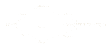
It is not definitionally the condensed spectrum in equation (26). The parameter sites, gap witnesses, lattice conventions, and descent conditions differ. A comparison should first be defined on their common smooth, uniformly controlled domain.

Aoki’s K-theory bridge

Aoki proves, with connective and Bott-periodic qualifications, that solidification of algebraic K-theory of real or complex Banach algebras recovers the corresponding connective topological K-theory, followed by inversion of the degree-two complex or degree-eight real Bott element for the periodic theory. This is an Established invariant-level bridge [Aoki2024].

The input Banach or C*-algebra is already present. Solidification does not recover its norm, positive cone, state space, or microscopic interaction. It also does not say that every K-class is a physical phase.

Comparison diagram

The honest current diagram is

Three realized low-dimensional rows

The companion realizability analysis establishes three concrete rows.

Each row is microscopically realized in the stated one-dimensional setting. The last column records a limited comparison, not a spectrum equivalence.

Surjectivity and injectivity

Surjectivity of a realization map would require every abstract class to have a local Hamiltonian witness with a uniform gap and the correct response. Anomalies, finite-dimensional local Hilbert spaces, spatial symmetry, or unknown gap proofs may obstruct or delay such a result.

Injectivity would require two systems with the same abstract class to be connected by the chosen stabilized gapped path. A field-theory target may forget crystalline data, noninvertible excitations, boundary termination, or unstable finite-band structure. If the microscopic category retains any of these, injectivity can fail.

The BDI example shows that changing the domain can also merge classes. Once interactions are admitted, paths exist that were absent in the free category. Realization and comparison questions are meaningless until the domain and its morphisms are fixed.

Package I: analytic family control

The first package should formulate a category of lattices and interactions on which a common locality norm implies family-uniform Lieb-Robinson bounds, thermodynamic dynamics, and restriction stability. It should include moving defects, disorder hulls, and variable local Hilbert spaces without confusing local continuity with uniform decay.

The main target is a base-change theorem: pullback of a controlled family preserves every constant used by the dynamics. A second target is finite descent for quantitative locality certificates. Infinite descent will need a bornological or boundedness condition that prevents constants from escaping.

Package II: gap certificates and openness

The second package should compare finite-volume and GNS witnesses under explicit boundary and sector hypotheses. Its output should be a stack of witnesses over the Hamiltonian moduli object, together with a theorem that the propositional image is pullback-stable.

A useful certificate has fields for the lower bound, volume threshold, ground-state sector, boundary convention, and theorem provider. This makes the gap claim transportable without pretending that the provider is unique.

Package III: phase localization

The third package should define controlled gapped paths, quasi-local automorphisms, finite-depth circuits, lattice changes, and stabilization in one infinity-categorical model. Comparison functors between these notions should be theorems, not definitional equalities.

The practical question is whether local phase equivalences glue. On an overlap, two spectral-flow providers may differ by a phase automorphism. That difference belongs in the higher groupoid and cannot be erased during descent.

Package IV: stacking and spectrification

The fourth package should prove that stacking preserves locality and gap witnesses with controlled constants, descends through localization, and is coherently symmetric monoidal. It should then distinguish actual physical inverses from formal Grothendieck inverses.

Connective spectrification is only part of the job. To compare spatial dimensions, one needs a theorem that adding a lattice direction implements the loop or suspension maps of an Omega-spectrum. Kubota’s construction is the clearest established benchmark for this step.

Package V: comparison and realization

The fifth package should build natural transformations on carefully chosen overlaps:

1. from free condensed Hamiltonian families to operator K-theory;

2. from Kubota’s smooth microscopic families to condensed tests;

3. from controlled microscopic invertible phases to reflection-positive effective field theories;

4. from a generalized cohomology invariant to relative transition classes;

5. from abstract classes back to explicit microscopic witnesses where possible.

Each map should list the information it forgets. A realization theorem should state its locality, symmetry, dimensional, and boundary restrictions.

Local interaction record

A local interaction family record contains $$\begin{equation} (\Gamma,d,\mathcal A_{\mathrm{loc}},\Phi,F,C_F,T_F,G,\alpha), \end{equation}$$ where $C_F$ is a common interaction-norm bound and $T_F$ is a common tail certificate. Restriction may change the parameter object but may not weaken the declared bound silently.

Hamiltonian moduli record

A Hamiltonian moduli record adds a test site, object and morphism categories, restriction functors, descent data, and size conventions. The object record alone defines a sheaf of data at best. Higher moduli require mapping anima and coherent descent.

Gap record

A gap witness contains $$\begin{equation} (\gamma,L_0,\text{sector},\text{boundary},\text{provider}) \end{equation}$$ or its GNS analogue. The qualitative flag is the truncation of the existence of such a record. The flag never substitutes for the provider during an analytic proof.

Phase record

A phase record lists its allowed paths, local circuits, quasi-local automorphisms, lattice changes, ancillas, and symmetry rules. Two papers that use different records may obtain different phase sets without contradiction.

Spectrum record

A spectrum record lists the symmetric monoidal operation, unit, physical inverse witness, $E_\infty$ coherences, test-object descent, and spatial suspension maps. A sequence of abelian groups is not a substitute for this record.