Physical Realizability of Invertible Phase Classes

Spatial dimension and spacetime dimension

Throughout the paper,

$$\begin{equation} d=\text{spatial dimension}, \qquad n=d+1=\text{spacetime dimension}. \tag{1} \end{equation}$$

Hamiltonians and lattices are indexed by $d$. The tangential symmetry type in the Freed-Hopkins formula is indexed by $n$. Thus every comparison row must visibly apply the shift in equation (1). In particular, a one-dimensional chain has $d=1$ but contributes to a two-dimensional spacetime theory with $n=2$.

What this paper proves

The main result is a verified portfolio, not a surjectivity theorem.

The proof occupies sections 4 to 6. The last sentence is part of the theorem’s scope, not a disclaimer added after the fact.

Status language

We use four statuses for realization questions.

The absence of a known model gives status Open, never Obstructed.

Microscopic stabilized phases

Let $\Gamma$ be a lattice of bounded geometry. Each site $x$ carries a finite-dimensional Hilbert space $\mathcal H_x$, or a finite-dimensional graded local algebra in a fermionic formulation. A finite-range or uniformly almost-local interaction $\Phi$ assigns a self-adjoint local operator $\Phi(X)$ to each finite $X\Subset\Gamma$.

For a periodic sequence of finite volumes $\Lambda_L$, the uniform-gap condition used in the examples is

$$\begin{equation} \inf_{L\ge L_0} \left(E_{m_L+1}(H_{\Lambda_L})-E_{m_L}(H_{\Lambda_L})\right) \ge \gamma>0. \tag{3} \end{equation}$$

Here $m_L$ is the dimension of the prescribed low-energy sector. For a periodic chain with a unique ground state, $m_L=1$. For an open AKLT chain, the four edge states form the low-energy sector and the relevant bulk gap is the gap above that sector.

Two data represent the same stabilized phase if, after adding atomic product-state ancillas, they are joined by a symmetry-preserving path of interactions that remains uniformly local and satisfies equation (3) along the path. Invertibility means that stacking with some second datum is gapped-homotopic, after stabilization, to the chosen atomic phase.

Freed-Hopkins deformation classes

Fix a spacetime symmetry type $(H_n,\rho_n)$, where $\rho_n:H_n\to O_n$ has compact internal kernel. Let $MTH$ be its Madsen-Tillmann spectrum and let $I\mathbb Z(1)$ denote the indicated Anderson-dual target.

The theorem is a field-theory classification. It is not a theorem that each element of equation (4) has a finite-range lattice Hamiltonian. The broader extension to all nontopological reflection-positive invertible theories is also not silently imported here.

Kubota’s microscopic Omega-spectrum

The objects in this theorem include a chosen nondegenerate gapped GNS ground state. Compact Lie on-site symmetry yields the stated naive equivariant variant. This should not be upgraded without proof to a genuine representation-graded equivariant spectrum.

The proposed condensed spectrum

A condensed moduli stack would evaluate parameterized Hamiltonian families on profinite or more general condensed test objects. Its invertible sector could then be group-completed and stabilized. This is a useful proposed target for disorder and inverse-limit parameter spaces. It is not Kubota’s smooth-manifold sheaf and it is not the bordism spectrum in theorem 2.3.

The current comparison situation is therefore

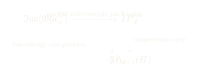
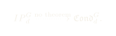
Solid arrows would require definitions on a common domain and proofs of continuity, symmetry compatibility, stabilization compatibility, and homotopy invariance. The dotted arrows in equation (5) are research questions.

Witness columns

The row is complete only if every required field is populated. Numerical evidence from finitely many lengths is not a uniform-gap theorem.

The verified low-dimensional matrix

Each row has microscopic status Realized. Its last column states a more limited comparison claim. The word “agreement” does not mean that the three spectra in equation (5) have been identified.

Hamiltonian and symmetry

On a chain of $L$ complex fermions, let $c_j,c_j^*$ satisfy the canonical anticommutation relations. With periodic or open boundary convention as specified, set

$$\begin{align} H_D(\mu,t,\Delta) ={}&-\mu\sum_j\left(c_j^*c_j-\frac12\right) -t\sum_j\left(c_j^*c_{j+1}+c_{j+1}^*c_j\right) \notag\\ &+\Delta\sum_j\left(c_jc_{j+1}+c_{j+1}^*c_j^*\right), \tag{6} \end{align}$$

where $t,\Delta\in\mathbb R$. Fermion parity $(-1)^F$ is exact. In BdG form, particle-hole conjugation is intrinsic and squares to $+1$. No time-reversal symmetry is imposed, so the system is in class D.

Introduce Majorana operators

$$\begin{equation} a_j=c_j+c_j^*, \qquad b_j=\frac{c_j-c_j^*}{i}. \end{equation}$$

At the solvable point $\mu=0$ and $\Delta=t>0$, an open chain has

$$\begin{equation} H_D=it\sum_{j=1}^{L-1}b_j a_{j+1}, \tag{8} \end{equation}$$

up to the conventional overall normalization. The operators $a_1$ and $b_L$ do not occur in equation (8). They form the two boundary Majorana zero modes.

Uniform periodic gap

For a periodic chain, the BdG symbol may be chosen as

$$\begin{equation} h_D(k)=(-\mu-2t\cos k)\tau_z+2\Delta\sin k\,\tau_y. \tag{9} \end{equation}$$

Here the Nambu spinor is $\Psi_k=(c_k,c_{-k}^*)^{\mathsf T}$. The matrices $\tau_y$ and $\tau_z$ are Pauli matrices in this ordered particle-hole basis, with the pairing phase chosen so that real $\Delta$ multiplies $\tau_y$.

Its positive quasiparticle energy is

$$\begin{equation} E(k)=\sqrt{(\mu+2t\cos k)^2+4\Delta^2\sin^2 k}. \tag{10} \end{equation}$$

The microscopic invariant

At the particle-hole fixed momenta $k=0,\pi$, the class-D invariant can be written as the sign of a product of Pfaffians. In the convention of equation (9),

$$\begin{equation} \nu_D=\operatorname{sgn}\bigl((\mu+2t)(\mu-2t)\bigr)\in\{+1,-1\}. \tag{12} \end{equation}$$

Thus $|\mu|<2|t|$ gives $\nu_D=-1$. The solvable point lies in this region. The open-chain boundary Majoranas supply a second diagnostic of the same phase.

Comparison status

In spacetime dimension $n=2$, the corresponding invertible spin field theory is the nontrivial Arf theory. Both the microscopic interacting class-D classification and this low-dimensional field-theory sector are $\mathbb Z_2$. The Kitaev chain is the standard microscopic representative of the nontrivial element.

This agreement is strong evidence for the expected low-energy comparison. It does not define the dotted arrow in equation (5) on all microscopic phases, parameter families, or dimensions.

Free integer index

Take $r$ copies of the real Kitaev chain. Let the antiunitary symmetry $T$ act by complex conjugation in the real-fermion basis, so that

$$\begin{equation} T i T^{-1}=-i, \qquad T c_{j,\alpha}T^{-1}=c_{j,\alpha}, \qquad T^2=+1. \tag{13} \end{equation}$$

Together with BdG particle-hole structure this is class BDI. The real off-diagonal symbol has an integer winding number. A stack of $r$ solvable chains has

$$\begin{equation} \nu_{\mathrm{free}}=r\in\mathbb Z \end{equation}$$

and carries $r$ Majorana zero modes at each open end. Its periodic bulk gap is again $2t$.

Why the integer is not an interacting invariant

The interaction is local and quartic in the boundary Majoranas, and its bulk extension supplies the gapped interpolation. The cited construction, not a finite-size numerical extrapolation, is the gap witness for the reduction. For eight stacked chains, write $\gamma_a$ for the eight unpaired boundary operators selected from the $a_j,b_j$ basis used in equation (8). At an end where these $\gamma_a$ are $T$-even, a monomial $\gamma_a\gamma_b\gamma_c\gamma_d$ with a real coefficient is also $T$-even and preserves fermion parity. The Fidkowski-Kitaev interaction is built from such quartic terms, so the mechanism gaps the boundary multiplet without violating equation (13).

Pin structure and the abstract class

The antiunitary relation $T^2=+1$ for the BDI fermion corresponds to the $\mathrm{Pin}^-$ tangential structure in two spacetime dimensions. The Arf-Brown-Kervaire invariant has values in $\mathbb Z_8$, matching equation (15). This is a particularly sharp low-dimensional agreement between microscopic interaction reduction and bordism data.

The comparison still uses the low-energy field-theory interpretation in theorem 2.3. It is not a construction of a natural equivalence between Kubota’s $\mathit{IP}_*$ and the Freed-Hopkins mapping spectrum.

Interaction and symmetry

At each site place the spin-1 irreducible representation of $SO(3)$. Write $\mathbf S_j=(S_j^x,S_j^y,S_j^z)$. For neighboring sites let $P^{(2)}_{j,j+1}$ be the orthogonal projection onto total spin two. Since $x=\mathbf S_j\cdot\mathbf S_{j+1}$ has eigenvalues $-2,-1,1$ in total-spin sectors zero, one, and two,

$$\begin{equation} P^{(2)}_{j,j+1} =\frac16\left( (\mathbf S_j\cdot\mathbf S_{j+1})^2 +3\mathbf S_j\cdot\mathbf S_{j+1} +2 \right). \tag{16} \end{equation}$$

The AKLT Hamiltonian is

$$\begin{equation} H_{\mathrm{AKLT}}=\sum_j P^{(2)}_{j,j+1}. \tag{17} \end{equation}$$

Every term is a positive nearest-neighbor projection. The diagonal on-site $SO(3)$ action commutes with each term.

Ground states, edges, and bulk gap

The valence-bond construction represents each spin one as the symmetric subspace of two virtual spin-$1/2$ variables and pairs neighboring virtual spins into singlets. On a periodic chain it gives the unique ground state. On an open chain, one virtual spin-$1/2$ remains at each boundary, giving a four-dimensional ground-state sector.

This is the imported gap theorem for the row. Frustration freeness alone would not have been enough.

Projective boundary invariant

The physical spin-1 representation descends from $SU(2)$ to a linear representation of $SO(3)$. A single virtual edge spin transforms in the spin-$1/2$ representation of $SU(2)$. The central element $-1\in SU(2)$ acts on it as $-\mathrm{id}$, so this action does not descend to a linear representation of $SO(3)$. It defines the nontrivial projective class

$$\begin{equation} [\omega_{\mathrm{edge}}] \in H^2(SO(3),U(1))\cong\mathbb Z_2. \tag{18} \end{equation}$$

The same $\mathbb Z_2$ appears in the low-dimensional bosonic field-theory sector with $SO(3)$ background. As in the fermionic examples, this row checks a generator and not the essential surjectivity of a general comparison functor.

The exact sequence of a pair

Let $E$ be a multiplicative generalized cohomology theory represented by a spectrum. Let $B$ be a space in a category where the pair axiom and excision hold, and let $\Sigma\subset B$ be closed. Put $U=B\setminus\Sigma$. We assume the inclusions have been replaced by cofibrant pairs when necessary, so that the cofiber model computes relative cohomology.

The pair $(B,U)$ has the long exact sequence

$$\begin{equation} \cdots\longrightarrow E^q(B) \xrightarrow{j^*}E^q(U) \xrightarrow{\partial}E^{q+1}(B,U) \xrightarrow{i^*}E^{q+1}(B) \longrightarrow\cdots. \tag{19} \end{equation}$$

The converse concerns extension in the chosen cohomology theory. It does not say that a Hamiltonian family itself extends across $\Sigma$ while remaining gapped.

Excision near the gapless locus

This theorem is the precise sense in which equation (20) is supported near $\Sigma$.

Thom identification

Suppose now that $B$ is a smooth manifold and $\Sigma\hookrightarrow B$ is a closed smooth submanifold of codimension $c$. Let $\mathcal N\to\Sigma$ be its normal bundle. Assume $\mathcal N$ is $E$-oriented, meaning it has a Thom class

$$\begin{equation} u_E\in\widetilde E^c(\operatorname{Th}(\mathcal N)) \end{equation}$$

whose restriction to every normal fiber is a generator in the required sense.

Without an $E$-orientation, the last line must use the corresponding twisted cohomology. Omitting that twist can change or destroy the purported charge.

Linking spheres

At a point $x\in\Sigma$ where the normal bundle is locally trivial, restrict the Thom representative to a normal disk $D^c$ and its boundary $S^{c-1}$. The resulting local class measures the obstruction on a linking sphere. For ordinary cohomology this is the familiar local degree. For K-theory or another spectrum it is the corresponding generalized cohomology class.

Naturality required for physics

Suppose a microscopic family $H$ on $U$ has an invariant $\nu_{\mathrm{mic}}(H)$. To interpret equation (20) physically, one needs a natural transformation

$$\begin{equation} \kappa:\nu_{\mathrm{mic}}(H)\longmapsto \nu_E(H)\in E^q(U) \tag{24} \end{equation}$$

that is invariant under the chosen gapped homotopies and compatible with restriction to open sets. Naturality then makes the connecting morphism commute with the microscopic restriction maps.

The proposition is conditional. A relative group by itself does not create the microscopic map $\kappa$.

Restricted model portfolio

All verified rows are one-dimensional. They do not test chiral phases in two spatial dimensions, intrinsic topological order, noninvertible phases, or higher-form symmetry. The AKLT row is a spin system, while the class-D and BDI rows are fermionic. Moving between these settings can involve a choice of graded tensor product or Jordan-Wigner transformation and is not treated as invisible.

No general field-theory emergence theorem

We do not prove that a gapped lattice model has a relativistic infrared limit, that its low-energy theory is fully extended, or that this theory is faithful to microscopic phase equivalence. These are among the assumptions needed to apply theorem 2.3 to lattice systems.

No surjectivity

Nothing here proves that every element of $[MTH,\Sigma^{n+1}I\mathbb Z(1)]_{\mathrm{tors}}$ is realized by a local Hamiltonian. Nothing proves that every homotopy class in a proposed condensed spectrum comes from Kubota’s construction, or conversely.

Boundaries and degeneracy

Uniform bulk gaps and open-boundary spectral gaps are different statements. We explicitly retain the low-energy edge sector in equation (3). Boundary perturbations can split that sector while leaving the bulk gap open. A realizability row must state which notion it uses.

Relative charge needs orientation and comparison

The Thom identification in equation (23) can fail without an $E$-orientation of the normal bundle. Excision can fail if one works outside a category of good pairs without a supported-cohomology replacement. Most importantly, a relative generalized cohomology class is not automatically measurable until the microscopic invariant and response map are specified.

A useful next theorem

A major next step would be a natural transformation from a controlled microscopic invertible phase spectrum to an Anderson-dual bordism target, defined on smooth parameter families and compatible with stacking, suspension, spatial symmetry, and spectral flow. Its value on the three rows in this paper should recover the stated low-dimensional comparisons. Constructing that map is Open.

Class D

BDI

AKLT